Lens Potential and Basic Notation

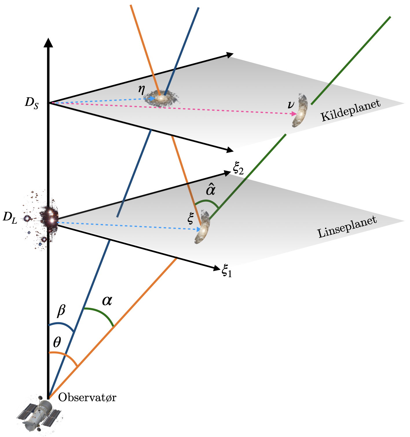
We assume a flat sky, so that the source is contained in a plane $S$ at distance $D_S$ from the observer, and the lens in a plane $L$ at distance $D_L$ from the observer. The optical axis is the line from the observer through the lens. The planes $S$ and $L$ are orthogonal on the optical axis, and have origin in the intersection therewith.

We consider a single source point at $\boldsymbol{\eta}$ in $S$. The apparent position, as seen by the observer, is at $\nu$ and \begin{equation} \Delta\boldsymbol{\eta} = \boldsymbol{\nu} - \boldsymbol{\eta} \end{equation} The apparent position in the lens plane $L$ is called \begin{equation} \boldsymbol{\xi} = \frac{D_L}{D_S} \boldsymbol{\nu}. \end{equation}

The deflection is most easily described in terms of angles, so we define $\beta$ and $\theta$ as the angles between the optical axis and respectively $\boldsymbol{\eta}$ and $\boldsymbol{\nu}$. The deflection angle $\hat\alpha$ is the angle between the actual and apparent source in the source plane as seen from the apparent image in the lens plane.

With the flat sky approximation, the angles are related to lengths in the lens plane by a factor of $D_L$, so that \begin{align} \boldsymbol{\xi} & = D_L\theta \end{align} Similarly, in the source plane, the factor is $D_S$ \begin{align} \boldsymbol{\nu} & = D_S\theta \\\
\boldsymbol{\eta} & = D_S\beta \\\
\Delta\boldsymbol{\eta} & = D_S\alpha \end{align} where $\alpha=\theta-\beta$ as the angle between $\boldsymbol{\eta}_S$ and $\boldsymbol{\nu}_S$ as seen from the observer. The same reasoning gives us the following¹,

\begin{equation} \alpha = \frac{D_{LS}}{D_S} \hat\alpha \end{equation}

Now, we can write the actual image as \begin{equation} \boldsymbol{\eta} = \frac{D_S}{D_L}\boldsymbol{\xi} - D_{LS}\boldsymbol{\hat\alpha} \end{equation}

Normalisation

The above definitions assume physical units. It is customary to normalise using a constant factor $\xi_0$, corresponding to the Einstein radius. This gives the following entities, following Kormann 1994²

\begin{align} \mathbf{x} & = \frac{\boldsymbol{\xi}}{\xi_0} \\\
\mathbf{y} & = \frac{\boldsymbol{\eta}}{\eta_0} \quad\text{where } \nu_0 = \frac{D_S}{D_L}\xi_0 \\\
\mathbf{a} & = \frac{D_LD_{LS}}{D_S\xi_0}\hat{\boldsymbol{\alpha}} = \frac{D_L}{\xi_0}\boldsymbol{\alpha} \end{align}

The Einstein radius is a distance in the lens plane. The corresponding angle is $\xi_0/D_L$ which is used to denormalise $\mathbf{a}$ above.

The lens potential (gravitational potential) can be written as a function $\psi$ of either the angle $\theta$, the vector $\boldsymbol{\xi}$, or the normalised $\mathbf{x}$. The normalised deflection $\mathbf{x}$ is given as the gradient of $\psi$, i.e. \begin{equation} \mathbf{a} = \nabla_{\mathbf{x}}\psi \end{equation} Different forms of $\psi$ give³, \begin{align} \mathbf{a} = \xi_0\cdot\nabla_{\xi}\psi = \frac{\xi_0}{D_L}\cdot\nabla_{\theta}\psi \end{align}

The Raytrace Equation

The normalised raytrace equation is given as \begin{align} \mathbf{y} = \mathbf{x} - \mathbf{a} \end{align} Inserting the gradient for $\mathbf{a}$, we have \begin{align} \mathbf{y} = \mathbf{x} - \nabla_{\mathbf{x}}\psi \end{align} We can rewrite the raytrace equation using any of the forms of $\nabla\psi$. In terms of $\xi$, we have \begin{equation} \boldsymbol{\eta} = \frac{D_S}{D_L}\boldsymbol{\xi} - D_{LS}\boldsymbol{\hat\alpha} = \frac{D_S}{D_L}(\boldsymbol{\xi} - \xi_0\mathbf{a}) = \frac{D_S}{D_L}(\boldsymbol{\xi} - \xi_0^2\nabla_{\xi}\psi) \end{equation} In terms of angles, we have \begin{equation} \boldsymbol{\beta} = \theta - \alpha = \theta - \frac{\xi_0}{D_L}\mathbf{a} = \theta - \frac{\xi_0}{D_L}\mathbf{a} = \theta - \frac{\xi_0^2}{D_L^2}\nabla_{\theta}\psi \end{equation}

Lens Potential in CosmoSim

In the implementation of CosmoSim, we have used a different definition of $\psi$, \begin{equation} \psi^{\mathrm{R}} = \frac{\xi_0^2}{D_L^2}\psi \end{equation} TODO double-check this

In this notation, we can write the raytrace equation as \begin{equation} \boldsymbol{\eta} = \frac{D_S}{D_L}(\boldsymbol{\xi} - \nabla_{\xi}\psi^{\mathrm{R}}) = \boldsymbol{\nu} - \frac{D_S}{D_L} \nabla_{\xi}\psi^{\mathrm{R}} \end{equation} This is relation is implemented in the RaytraceModel::calculateEta() function in CosmoSim.

Surface Mass Density

The convergence, or dimensionless projected surface-mass density, is given as a function $\kappa$, which is related to $\psi$ as follows: \begin{equation} \kappa(\boldsymbol{\xi})= \frac12\xi_0^2\left( \frac{\partial^2\psi}{\partial\xi_1^2} + \frac{\partial^2\psi}{\partial\xi_2^2} \right) \end{equation} or \begin{equation} \kappa(\boldsymbol{\xi})= \frac12D_L^2\left( \frac{\partial^2\psi^{\mathrm{R}}}{\partial\xi_1^2} + \frac{\partial^2\psi^{\mathrm{R}}}{\partial\xi_2^2} \right) \end{equation}

Notes

1. This is seen because $D_S\alpha$ and $D_{LS}\hat\alpha$ are the lengths of arcs between the actual and apparent source, and for small angles they are both approximately equal to the straigh line $\Delta\boldsymbol{\eta}_S$. ↩

2. Kormann uses $\boldsymbol{\alpha}$ for $\mathbf{x}$, but we have already used that for $\theta-\beta$. ↩

3. We use here the chain rule with $\boldsymbol{\xi}= \xi_0\mathbf{x} $ and $\theta = \boldsymbol{\xi}/D_L$. ↩