The Roulette Formalism

DRAFT under construction

\begin{equation} \alpha_s^m = - \frac{1}{2^{\delta_{0s}}} D_\textrm{L}^{m+1} \sum_{k=0}^m\binom{m}{k} \left(\mathcal{C}_s^{m(k)}\partial_{\xi_1}+\mathcal{C}_s^{m(k+1)}\partial_{\xi_2}\right) \partial_{\xi_1}^{m-k}\partial_{\xi_2}^k\psi \end{equation}

\begin{equation} \mathcal{C}_s^{m(k)}=\frac{1}{\pi}\int_{-\pi}^{\pi}{\rm d}\phi\sin^k\phi\cos^{m-k+1}\phi\cos s\phi \end{equation}

\begin{equation} \beta_s^m=-D_\textrm{L}^{m+1}\sum_{k=0}^m\binom{m}{k}\left({\mathcal{S}}_s^{m(k)}\partial_{\xi_1}+{\mathcal{S}}_s^{m(k+1)}\partial_{\xi_2}\right)\partial_{\xi_1}^{m-k}\partial_{\xi_2}^k\psi \end{equation}

\begin{equation} \mathcal{S}_s^{m(k)}=\frac{1}{\pi}\int_{-\pi}^{\pi}{\rm d}\phi\sin^k\phi\cos^{m-k+1}\phi\sin s\phi. \end{equation}

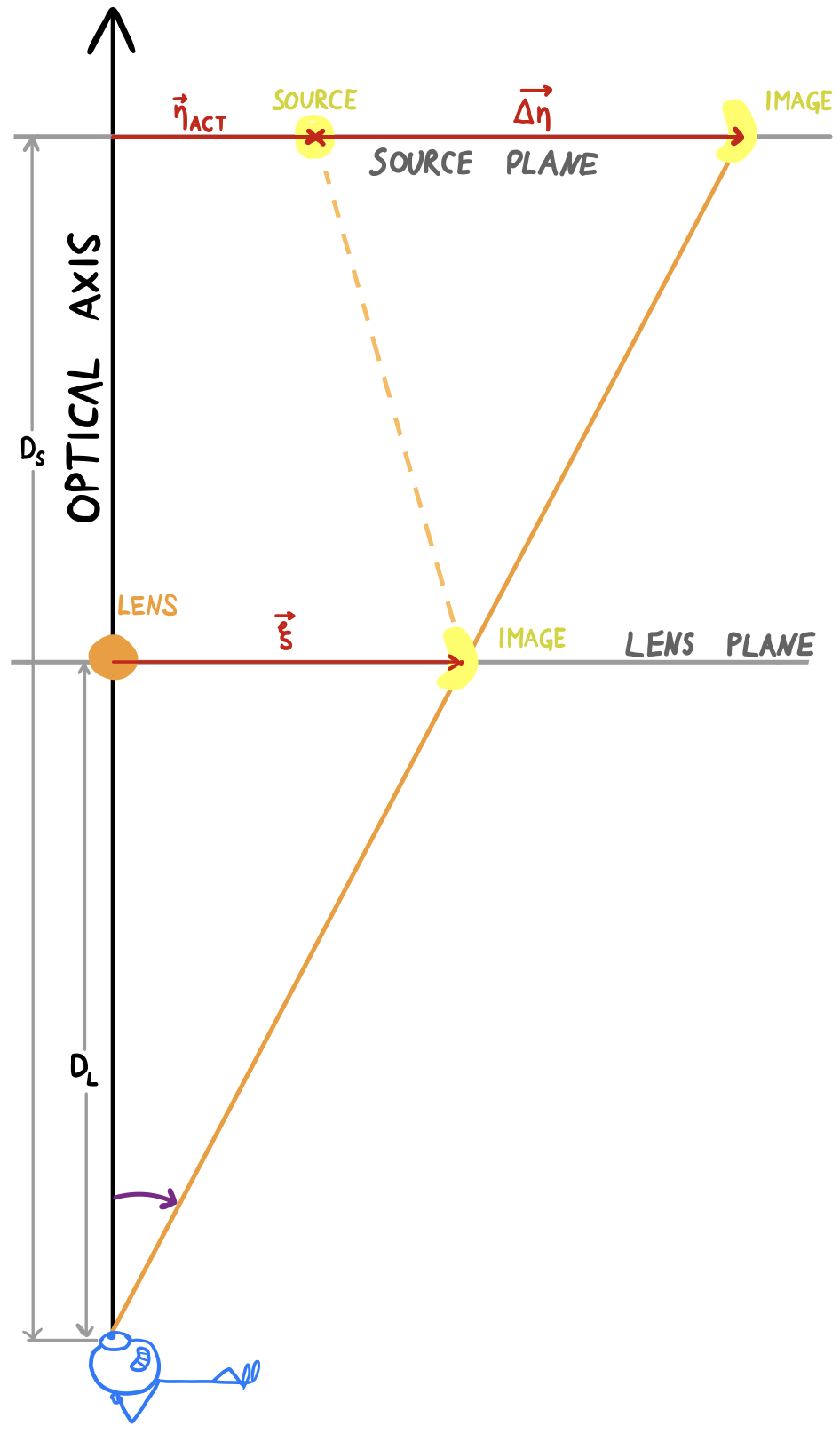
The observed lensing is decomposed into two steps, as shown the figure. The first step is a translation (deflection), corresponding to the difference $\boldsymbol{\Delta\eta}$ between actual ($\boldsymbol{\eta}_\textrm{act}$) and apparent ($\boldsymbol{\eta}_\textrm{app}$) source-plane position. In the roulette formalism, this translational part of the lensing is given as \begin{equation} \boldsymbol{\Delta\eta} =\boldsymbol{\eta}_\textrm{app}-\boldsymbol{\eta}_\textrm{act} =-D_\textrm{S}\cdot(\alpha^0_1,\beta^0_1), \end{equation} where $(\alpha^0_1,\beta^0_1)$ is a vector of roulette amplitudes, as defined above.

The second step is the actual, non-linear distortion. The distorted image is drawn in a local co-ordinate system in the lens plane, centred at $\boldsymbol{\xi}=(\xi_1,\xi_2)$, which corresponds to $\boldsymbol{\eta}_\textrm{app}$ in the source plane. We write $\xi=|\boldsymbol{\xi}|$ for the distance between the distorted image and the lens in the lens plane. Since $\boldsymbol{\xi}$ and $\boldsymbol{\eta}_{\mathrm{app}}$ lie on the same line through the viewpoint (cf. figure), we have \begin{equation} \xi = |\boldsymbol{\xi}| = \frac{D_\textrm{L}}{D_\textrm{S}}\cdot|\boldsymbol{\eta}_{\mathrm{app}}|. \end{equation} Following Clarkson, we use polar co-ordinates $(r,\phi)$ for the distorted image. The source image is described in Cartesian co-ordinates $(x^\prime,y^\prime)$ centered at $\boldsymbol{\eta}_\textrm{act}$ in the source plane. Thus the light observed at a position (pixel) $(r,\phi)$ is drawn from a different position (pixel) $(x’,y’)=\mathcal{D}$$(r,\phi)$ in the source image. From~Eq.~48 in \citet{Clarkson_2016_II} it is possible to show that the mapping $\mathcal{D}$ is given as \begin{aligned} \frac{D_{\mathrm{L}}}{D_{\mathrm{S}}}\cdot \begin{bmatrix} x’ \\ y’ \end{bmatrix} &= r\cdot\begin{bmatrix} \cos\phi \\ \sin\phi \end{bmatrix} + \sum_{m=1}^{\infty} \frac{r^m}{m!\cdot D_{\mathrm{L}}^{m-1}} \cdot\sum_{s=0}^{m+1} c_{m+s} \left(\alpha_s^m \boldsymbol{A}_{s} + \beta_s^m \boldsymbol{B}_{s} \right) \begin{bmatrix} C^+ \\ C^- \end{bmatrix} \\\
C^\pm &= \pm \frac{s}{m+1},\\\
c_{m+s} &= \frac{1 - (-1)^{m+s}}{4} = \begin{cases} 0, \quad m+s \text{ is even},\\\
\frac12, \quad m+s \text{ is odd}, \end{cases} \\\
\boldsymbol{A}_{s} &= \begin{bmatrix} \cos{(s-1)\phi} & \cos{(s+1)\phi} \\\
-\sin{(s-1)\phi} & \sin{(s+1)\phi} \end{bmatrix}, \\\
\boldsymbol{B}_{s} &= \begin{bmatrix} \sin{(s-1)\phi} & \sin{(s+1)\phi} \\\
\cos{(s-1)\phi} & -\cos{(s+1)\phi} \end{bmatrix}. \end{aligned} The coefficients $\alpha_m^s$ and $\beta_m^s$ depend on the lens potential $\psi(\xi_1,\xi_2)$, from which one may derive the physical properties of the lens.

In practice the sum has to be truncated by limiting $m\le m_0$ for some $m_0$.