Cluster Dataset (4x SIS) - CosmoSim Experiments July 2026

In this demo we show the generation of a dataset for machine learning sporting two SIE lenses. To run the notebook, you will have to download several datafiles from Experiment 3 (4xSIS).

Preparation¶

import pandas as pd
import matplotlib.pyplot as plt
import numpy as np
from PIL import Image
import json
from CosmoSim.datagen import SimImage
import CosmoSim.Image as csimg
import CosmoSim.dataset as csd
from CosmoSim import Parameters

The distribution of the dataset is configured as follows.

cfg = csd.readtoml( "cluster4-dataset.toml" )
display( json.dumps( cfg ) )

'{"simulator": {"model": "Raytrace", "size": 15000, "nterms": 4, "imagesize": 512, "cropsize": 256, "centred": true}, "dataset": {"directory": "images"}, "lens": {"mode": "SIS", "einstein-min": 3, "einstein-max": 75}, "cluster": {"count": 4, "maxrelativelocation": 1.2}, "source": {"mode": "SersicSphere", "n_sersic-min": 1, "n_sersic-max": 5, "luminosity-min": 20, "luminosity-max": 80, "luminosity-lambda": 2.0, "sigma-min": 5, "sigma-max": 50, "position": "critical"}, "position": {"phi-min": 0, "phi-max": 360, "r-relativemax": 1.2}}'

Each constituent lens is placed in a random direction from the origin, at a random distance upper bounded as $c\theta_E$ where $\theta_E$ is the Einstein radius and $c$ is the constant given as cluster.maxrelativelocation.

We can draw a random object as before.

A sample¶

Let us make a random sample for review. Firstly, we make a convenience function to run one simulation and retrieve the image.

def mkimg(ob):
      p0 = Parameters( )
      p0.setRow( ob )
      sim = SimImage( p0, verbose=0 )
      return sim.getImage()

Using this function, we can make a list of simulations, and plot the results.

obs = [ csd.getline( cfg ) for _ in range(8) ]
ims = [ mkimg(ob) for ob in obs ]
ts = [ f"Image {i}" for i in range(8) ]
csimg.showImages( ims, size=(2,4), titles=ts )

[getline] idx=0
[CosmoSim/py] setCluster(SIS/2.5313256566409277/2.156598485080758/19.491911132521416;SIS/33.442332645352316/-12.589891150146979/37.072213924898236;SIS/6.705942207614149/4.716244216548211/51.914626829879836;SIS/-20.732625090449236/-27.898030264417503/38.00719890582793)

[getline] idx=0
[CosmoSim/py] setCluster(SIS/-4.3822743297759725/3.4510887243354467/4.688828245157102;SIS/5.1800717619539665/3.7736421855758184/12.178693081449726;SIS/8.305646469379102/-11.934642075255013/17.52341679514656;SIS/-0.11857690120865512/-0.12211788517268332/22.854218944607624)

[getline] idx=0
[CosmoSim/py] setCluster(SIS/2.173465703186372/-26.217973168360267/22.49091180259033;SIS/-15.300468953458262/1.5544323582091553/35.10995805384463;SIS/0.5860453876361221/-6.411887628848669/33.239428885039864;SIS/-1.47641376229984/2.532535377534986/26.126169000769913)

[getline] idx=0
[CosmoSim/py] setCluster(SIS/14.378846920087414/-27.628165485550497/42.46821367734338;SIS/-1.7180669893353728/4.010374296282301/28.713986884060496;SIS/5.952751941883564/-14.491190928232434/65.75251917362509;SIS/-15.11287396919017/4.651405053955791/44.14308570218904)

[getline] idx=0
[CosmoSim/py] setCluster(SIS/-2.6893823632281793/-40.771017849447595/72.02236224076444;SIS/6.0928567293560265/-2.4570608426964062/29.689012220913057;SIS/-1.321102810769928/-0.9721070726722766/11.673714528778657;SIS/-28.54455588896845/4.401599370481382/35.64963382145919)

[getline] idx=0
[CosmoSim/py] setCluster(SIS/0.15042948427462458/-0.16852788653803358/5.681076434029771;SIS/-12.318952285591932/2.0443591269542654/29.68298478802107;SIS/3.6823890437459554/2.0751855133716375/18.474151233602015;SIS/-0.7256691299008825/0.3373390480008725/6.103332727840392)

[getline] idx=0
[CosmoSim/py] setCluster(SIS/52.010806736547075/-53.4403207501109/66.74523461209712;SIS/-5.330052864647665/-7.350314198216756/15.634950519441311;SIS/-5.78331682797284/12.92688034436884/15.331313560006967;SIS/1.2099139895233406/-4.196035445710545/31.56087987712155)

[getline] idx=0
[CosmoSim/py] setCluster(SIS/6.106585289889946/-10.010695194620588/10.843362458658628;SIS/-6.274811962517895/-21.238900782542483/37.53465652610117;SIS/0.06691066393321937/-0.5263888818151947/72.74019630962337;SIS/-2.846631574771813/-0.5982023702811042/55.48450679153229)

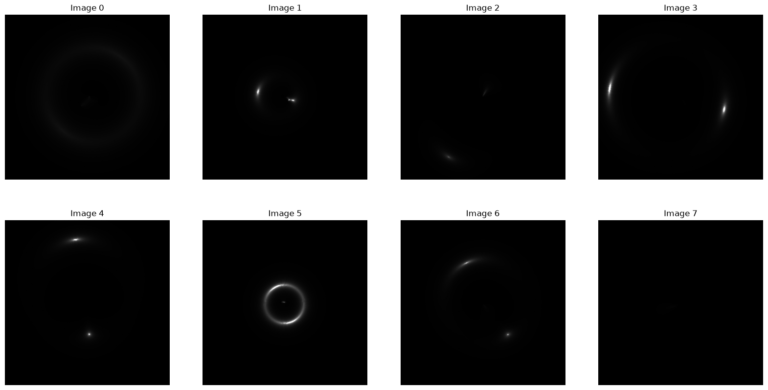
If we take a particular interest in one particular image, say no 1, we can easily inspect its parameters.

print( obs[1] )

index                                                         0
filename                                       image-000000.png
model                                                  Raytrace
cluster       SIS/-4.3822743297759725/3.4510887243354467/4.6...
source                                             SersicSphere
R                                                     29.789975
phi                                                  169.599211
sigma                                                  24.44496
sigma2                                                23.728767
theta                                                143.606781
n_sersic                                               4.598222
luminosity                                            76.577222
x                                                    -29.300496
y                                                      5.378064
dtype: object

The cluser specification does not show in the row view, but we can single that one out to see properly.

print( obs[1]["cluster"] )

SIS/-4.3822743297759725/3.4510887243354467/4.688828245157102;SIS/5.1800717619539665/3.7736421855758184/12.178693081449726;SIS/8.305646469379102/-11.934642075255013/17.52341679514656;SIS/-0.11857690120865512/-0.12211788517268332/22.854218944607624

Annotations¶

It may be interesting to look at the Critical Curves, to get an idea of the shape of the lenses. Instead of mkimg() we make a function to get annotated images.

def mkannotation(ob):
      p0 = Parameters( )
      p0.setRow( ob )
      sim = SimImage( p0, verbose=0 )
      return sim.getAnnotated()

We use the same datasets as before, but generate new and annotated images.

ims = [ mkannotation(ob) for ob in obs ]
csimg.showImages( ims, size=(2,4), titles=ts )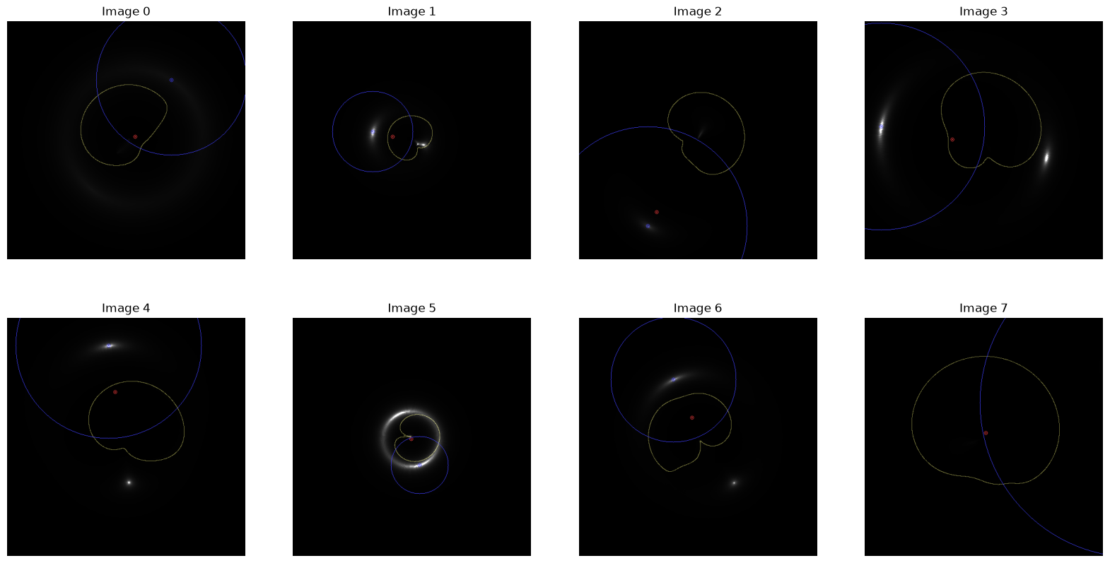

The yellow curve is the Critical Curve, and the blue circle is the convergence ring of the roulette formalism. The red point is the centre of light.

Closure¶

We have attemmpted to design the dataset so that it displays interesting samples of strong lensing.
More research is needed on actual distributions of observed lenses, and how a representative sample can be designed for machine learning.