Pointmass Demo - CosmoSim

The simplest lens model in CosmoSim is the pointmass, where all the mass is compressed in a singular point. This model is implemented many times. Currently, there is a PointMass lens which can be used with the standard models, RouletteModel and RaytraceModel. The original implementations PointMassRoulette and PointMassExact should be equivalent, but used a closed form specific to the point mass lens, and thus cannot be modularised.

Preparation¶

import pandas as pd
import matplotlib.pyplot as plt
import numpy as np
from PIL import Image
import toml

import CosmoSim as cs
from CosmoSim import CosmoSim, Parameters
from CosmoSim.datagen import SimImage
import CosmoSim.Image as csimg

print( "CosmoSim version:", cs.__version__ )

CosmoSim version: 3.1.2

The exact models¶

We can define the configuration as a dict using the nested (TOML) structure.

cfg = { 'simulator' : { "model" : "Raytrace", "cropsize" : 256 }
      , 'lens': { 
            'mode' : "PM",
            'einsteinR': 46,
            'ellipseratio': 0.34,
            'orientation': 107,
            'chi': 50}
      , 'source': {
            'mode': 'Spherical',
            'sigma': 7,
            'position': 'cartesian'}
      , 'position': {'x': 35, 'y': 15}
      }

param = Parameters( cfg )
imsim01 = SimImage( param, verbose=0 )
im01 = imsim01.getImage()

To run the same simulation with the legacy, exact model, we simply change the simulator setting and rerun.

param["simulator"]["model"] = "Point Mass (exact)" 
imsim02 = SimImage( param, verbose=0 )
im02 = imsim02.getImage()
csimg.imageCompare( im01, im02, "Modular Raytrace", 'Exact Point Mass')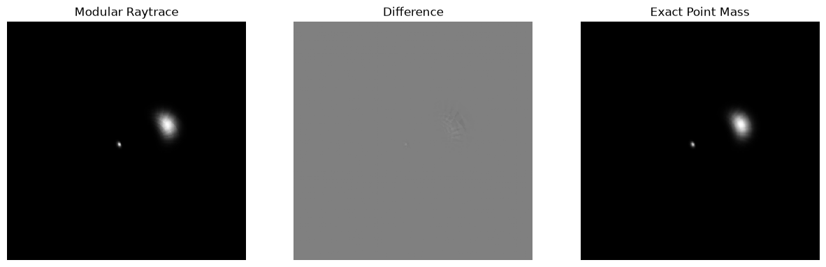

There is a visual discrepancy, but it is hard to tell if this is significant. Quite likely, it is due to numeric errors.

The original roulette¶

The roulette formalism is also implemented in a closed form.

param["simulator"]["model"] = "Point Mass (roulettes)"
param["simulator"]["nterms"] = 8
imsim03 = SimImage( param, verbose=0 )
im03 = imsim03.getImage()
csimg.imageCompare( im02, im03, "Exact Point Mass", 'Legacy Roulette')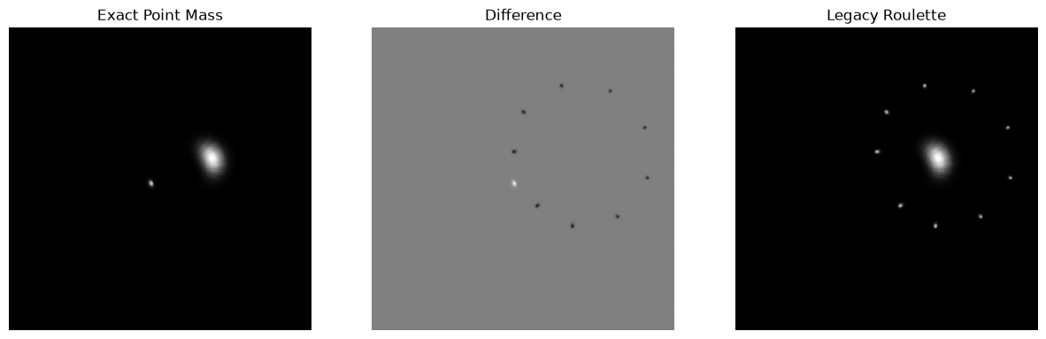

This looks perfect inside the convergence ring, as it should.

Modular roulette¶

param["simulator"]["model"] = "Roulette"
imsim04 = SimImage( param, verbose=0 )
im04 = imsim04.getImage()
csimg.imageCompare( im01, im04, "Modular Raytrace", 'Modular Roulette')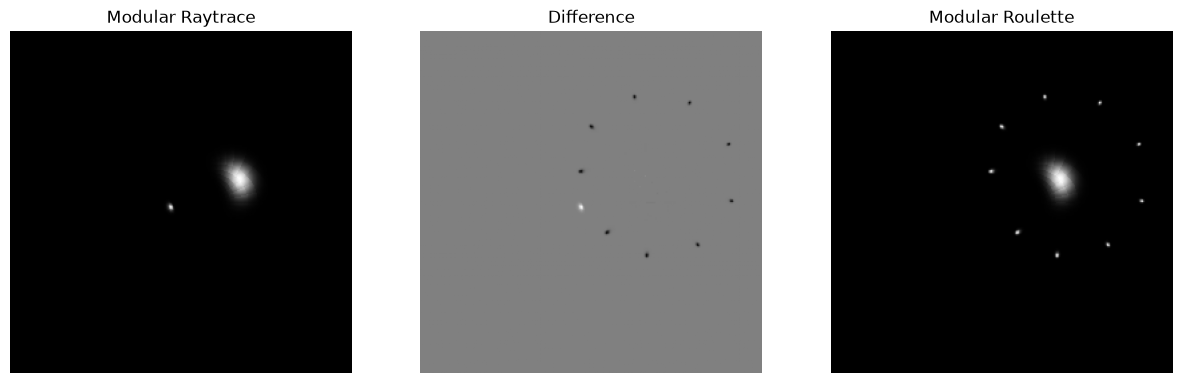

Again, the roulette simulation is perfect within the convergence ring.

If we compare the closed form and modular implementations, we find a discrepancy similar to what we had for the exact model and raytrace.

csimg.imageCompare( im03, im04, "Legacy Roulette", 'Modular Roulette')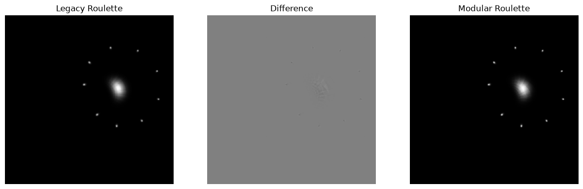

Sampling¶

The modular implementation allows for sampling and solution by numeric differentiation. Let us first test raytrace simulation and compare sampled and analytic solutions.

param["simulator"]["model"] = "Raytrace"
raytrace = SimImage( param, verbose=0 ).getImage()
param["simulator"]["sampled"] = True
raytraceS = SimImage( param, verbose=0 ).getImage()
csimg.imageCompare( raytrace, raytraceS, "Modular Raytrace", 'Sampled Raytrace')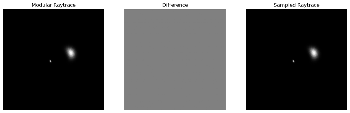

This looks perfect.

Then we can do the same with roulette.

param["simulator"]["model"] = "Roulette"
rouletteS = SimImage( param, verbose=0 ).getImage()
csimg.imageCompare( im04, rouletteS, "Modular Roulette", 'Sampled Roulette')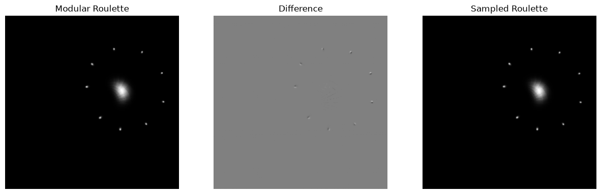

This gives a minor discrepancy in the spurious images, which may well be due to numeric approximation.

It is also useful to compare to the closed form implementations too.

csimg.imageCompare( im03, rouletteS, "Legacy Roulette", 'Modular Sampled Roulette')
csimg.imageCompare( im02, raytraceS, "Exact Point Mass", 'Modular Sampled Raytrace')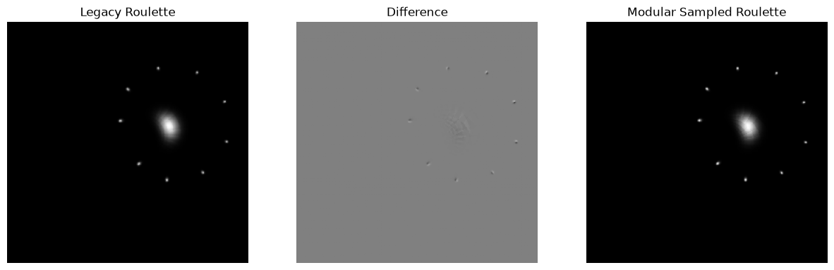

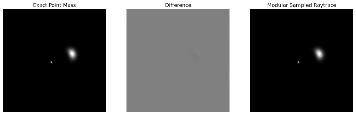
Here we have discrepancy similar to what we first saw between the closed form and modular implementations.

Rotation¶

The discrepancy that we have found may be due to rotation in the closed form implementation. We can test this by using a source on the $x$ -axis.

cfg = { 'simulator' : { "model" : "Raytrace", "cropsize" : 256 }
      , 'lens': { 
            'mode' : "PM",
            'einsteinR': 46,
            'ellipseratio': 0.34,
            'orientation': 107,
            'chi': 50}
      , 'source': {
            'mode': 'Spherical',
            'sigma': 7,
            'position': 'cartesian'}
      , 'position': {'x': 40, 'y': 0}
      }

param = Parameters( cfg )
rotM = SimImage( param, verbose=0 ).getImage()

param["simulator"]["model"] = "Point Mass (exact)" 
rotX = SimImage( param, verbose=0 ).getImage()
csimg.imageCompare( rotM, rotX, "Modular Raytrace", 'Exact Point Mass')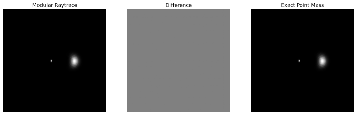

This is a perfect match as far as visiual perception goes. We can repeat the experiment with Roulettes.

param["simulator"]["model"] = "Roulette" 
param = Parameters( cfg )
rotMR = SimImage( param, verbose=0 ).getImage()

param["simulator"]["model"] = "Point Mass (roulettes)" 
rotR = SimImage( param, verbose=0 ).getImage()
csimg.imageCompare( rotMR, rotR, "Modular Roulette", 'Legacy Roulette')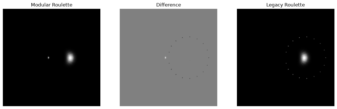

Again we have a perfect match.

Conclusion¶

We note that there is a discrepancy between the modular and closed form implementations, which may be due to the rotation of the image employed in the closed form implementations.

We also had a discrepancy in between the sampled and unsampled modular roulette impllementations, but this only affects the spurious images.