Evaluation of machine learning for SIE

This document evaluates one trained machine learning model, see details below. We use both conventional metrics and comparison with a resimulated image.

We use three datafiles, which must be downloaded if this document is to be executed.

sie-testing.csv is ground truth for model training
pred-sie-testing.csv is the predicted amplitudes from machine learning.
sie-dataset.csv is the original lens parameters used to generate the training, testing, and validation data, i.e. it has more rows than the other two sets.

The neural network used for machine learning is almost arbitrarily chosen and has not been tuned. The architecture is one of the best performing in Nicolò’s experiments on other datasets from CosmoSim, but the hyperparameters are arbitrarily chosen. The training set used is 16000 images.

The specification of the distribution is discussed in Sample Datasets for SIE and can be downloaded (sie-dataset.toml).

Configuration¶

import pandas as pd
import numpy as np
import matplotlib.pyplot as plt
from PIL import Image
import IPython.display as idp
import toml
import json
import CosmoSim.Image as csimg
import CosmoSim as cs
import CosmoSim.datagen as dg
import CosmoSim.roulettegen as rg
imshow = csimg.imshow
print( "CosmoSim version", cs.__version__ )

CosmoSim version 3.3.0

Let us check the parameters underlying this test. This gives the neural network and hyperparameters used.

cfg = toml.load( "ml.toml" )
print( "CosmoSim version is", cs.__version__ )
print( "Data from directory", cfg["output"]["directory"] )
print( "Neural network used:", cfg["settings"]["model"] )
print( json.dumps( cfg["hyperparameters"], indent=4 ) )

CosmoSim version is 3.3.0
Data from directory experiment001
Neural network used: regnet_y_32gf
{
    "learning-rate": 0.001,
    "batch-size": 32,
    "weight-decay": 0.0001
}

Let’s load the test set, both the ground truth (gt) and the predictions (df).

gt = pd.read_csv( "../sie-testing.csv", index_col="filename" )
df = pd.read_csv( "pred-sie-testing.csv", index_col="filename" )
display( gt.head() )
display( df.head() )

Loading...

As we can see, we have columns for all the parameters in question, and rows for the individual objects. There is no superfluous data in the data frames.

We can also check the difference.

rawerrors = gt - df
display( rawerrors.head() )

Loading...

That was straight forward. Now we come to the tricky part - making sense of the numbers. There are two questions that we want to consider.

How well does the model perform overall?
How do particular images behave, and what are the best and the worst samples?

Model evaluation¶

It is interesting to see how the model behaves on each column. To see this, we can aggregate the rows, computing the mean of absolute errors and mean of squared errors.

mse = (rawerrors**2).mean()
mae = rawerrors.abs().mean()
mse.name = "MSE"
mae.name = "MAE"
colerrors = pd.concat( [ mse, mae ], axis=1 )
display( colerrors )

Loading...

In practice, relative errors may be more interesting. We can calculate that too.

colerrors["mean"] = gt.abs().mean()
colerrors["Relative MAE"] = colerrors["MAE"] / colerrors["mean"]
display( colerrors )

Loading...

This looks good with mean relative errors less than 10^-7, and no column is particularly bad or good.

Object evaluation¶

To investigate individual objects, we start by calculating sum of squared errors for each one.

sse = (rawerrors**2).sum(axis=1)
display(sse)

filename
image-010001.png    9.425349e-12
image-010002.png    1.912532e-12
image-010003.png    3.255857e-11
image-010004.png    2.855730e-12
image-010005.png    6.062796e-12
                        ...     
image-013996.png    2.204224e-12
image-013997.png    2.924628e-12
image-013998.png    1.151700e-11
image-013999.png    3.498199e-12
image-014000.png    1.084519e-12
Length: 4000, dtype: float64

We can look at the three best and three worst images, thus,

sse.nlargest(3)

filename
image-012116.png    1.976053e-10
image-011292.png    1.665033e-10
image-012560.png    1.633072e-10
dtype: float64

sse.nsmallest(3)

filename
image-010843.png    2.397801e-15
image-013675.png    2.422658e-15
image-011485.png    4.103188e-15
dtype: float64

We note that the errors are small, but there is also a huge span between the best and the worst. For the purpose of this test, we do not assume that we have access to the original images, but we do have access to the lens parameters so that we can regenerate the images. First we record the filenames.

best = list(sse.nlargest(3).index)
worst = list(sse.nsmallest(3).index)
print( "Best:", best )
print( "Worst:", worst )

Best: ['image-012116.png', 'image-011292.png', 'image-012560.png']
Worst: ['image-010843.png', 'image-013675.png', 'image-011485.png']

Simulation from Roulette Amplitudes¶

Before we can simulate, we need to set up some basic parameters.

cfg = { "simulator" : { "imagesize" : 512
                      , "cropsize" : 256
                      , "xireference" : True
                      , "nterms" : 4 }
      , "source" : { "mode" : "SersicSphere" } }
param = cs.Parameters( cfg )

Lets first consider the worst images and the ground truth. The data is extracted as

gtw = gt.loc[ worst ]
display( gtw )

Loading...

To simulate, we instantiate the Resim class which is the simulator for roulette resimulation. For now, we test in just one image.

imsim = rg.Resim(gtw.iloc[0],param=param,verbose=0)
im = imsim.getImage()

[getSource] src=SersicSphere, ltprf0=None, verbose=1
[SphericalSource] constructor done

We can make the same simulation from the reconstructed amplitudes and compare the images.

dfw = df.loc[ worst ]
imsim2 = rg.Resim(dfw.iloc[0],param=param,verbose=0)
im2 = imsim2.getImage()
csimg.imageCompare( im, im2, "Ground Truth", "Reconstructed" )

[getSource] src=SersicSphere, ltprf0=None, verbose=1
[SphericalSource] constructor done

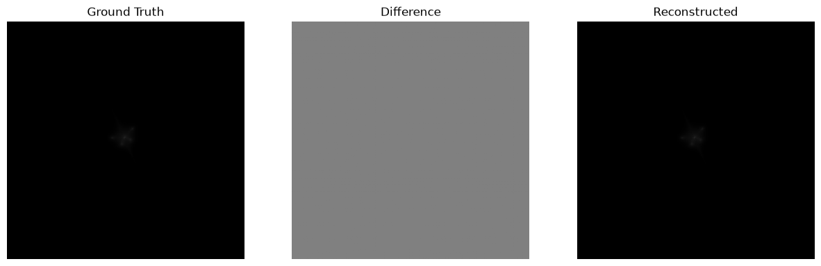
THis looks good, but the contrast is low, and the image may not be visible on all screens. In fact, I have reviewed this test on different screens, and devised the test below when working on a screen where this did look all black.

Dealing with low contrast images¶

When images look all black, it is worth investigating its parameters. First we identify the filename.

fn0 = worst[0]
print( fn0 )

image-010843.png

Then we can show the parameters.

display( df.loc[ worst[0] ] )

sigma          32.370200
luminosity     26.405500
n_sersic        1.668100
xiX            -2.254924
xiY             3.998422
alpha[0][1]     1.606023
beta[0][1]     -3.407914
alpha[1][0]    -0.147974
alpha[1][2]    -0.100855
beta[1][2]     -0.108280
alpha[2][1]    -0.019714
beta[2][1]      0.039949
alpha[2][3]    -0.042195
beta[2][3]      0.014146
alpha[3][0]    -0.008827
alpha[3][2]     0.007356
beta[3][2]      0.009573
alpha[3][4]    -0.002048
beta[3][4]      0.020753
alpha[4][1]    -0.003910
beta[4][1]      0.007948
alpha[4][3]     0.004565
beta[4][3]     -0.000921
alpha[4][5]     0.011710
beta[4][5]      0.006652
Name: image-010843.png, dtype: float64

This is rather low luminosity and large source size, which means that the light is spread out, and possibly faint. Let’s check the maximum pixel values.

dfsim = rg.Resim(df.loc[fn0],param=param,verbose=0)
dfim = dfsim.getImage()
gtsim = rg.Resim(gt.loc[fn0],param=param,verbose=0)
gtim = gtsim.getImage()
print( gtim.flatten().max(), dfim.flatten().max() )

[getSource] src=SersicSphere, ltprf0=None, verbose=1
[SphericalSource] constructor done

[getSource] src=SersicSphere, ltprf0=None, verbose=1
[SphericalSource] constructor done
34 34

Right, 34 is not far from black. We can boost the contrsst simply by multiplying by 4. We are still well within the 8-bit integer range.

csimg.imageCompare( dfim*4, gtim*4, fn0, "Ground Truth" )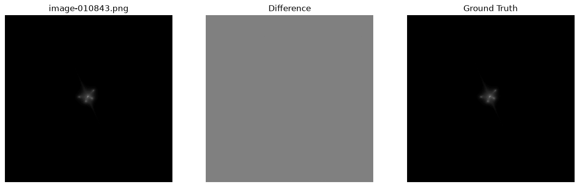

Now we can see the faint galaxy, and the match is perfect.

Full image set¶

We can do the same for all the top and bottom three.

for fn in worst:
    dfsim = rg.Resim(df.loc[fn],param=param,verbose=0)
    dfim = dfsim.getImage()
    gtsim = rg.Resim(gt.loc[fn],param=param,verbose=0)
    gtim = gtsim.getImage()
    csimg.imageCompare( dfim, gtim, fn, "Ground Truth", axiscross=True )
    plt.savefig( f"resim-{fn}" )

[getSource] src=SersicSphere, ltprf0=None, verbose=1
[SphericalSource] constructor done

[getSource] src=SersicSphere, ltprf0=None, verbose=1
[SphericalSource] constructor done

[getSource] src=SersicSphere, ltprf0=None, verbose=1
[SphericalSource] constructor done

[getSource] src=SersicSphere, ltprf0=None, verbose=1
[SphericalSource] constructor done

[getSource] src=SersicSphere, ltprf0=None, verbose=1
[SphericalSource] constructor done

[getSource] src=SersicSphere, ltprf0=None, verbose=1
[SphericalSource] constructor done

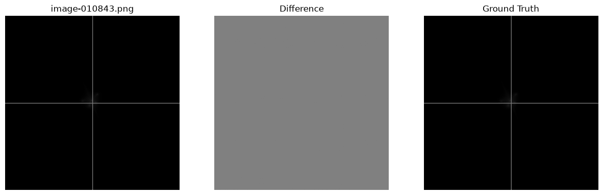
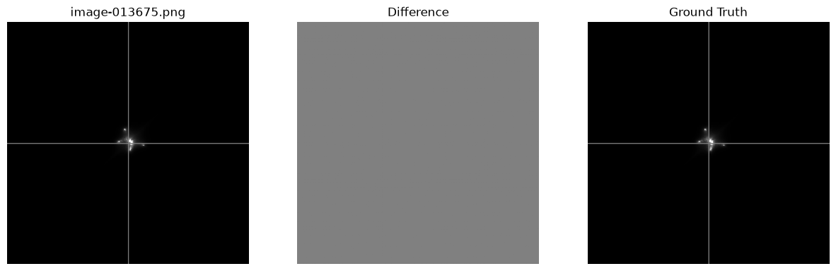
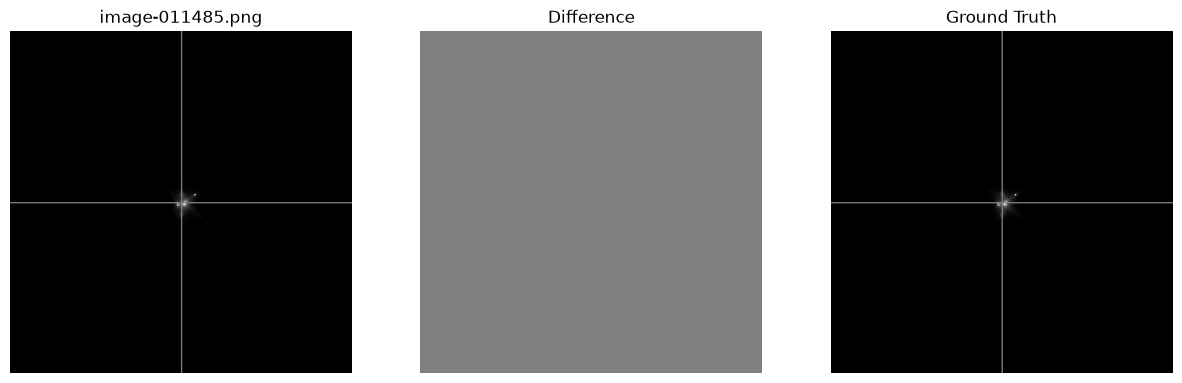
No visible discrepancy.

We can continue with the best images, obviously expecting perfect match again.

for fn in best:
    dfsim = rg.Resim(df.loc[fn],param=param,verbose=0)
    dfim = dfsim.getImage()
    gtsim = rg.Resim(gt.loc[fn],param=param,verbose=0)
    gtim = gtsim.getImage()
    csimg.imageCompare( dfim, gtim, fn, "Ground Truth" )
    plt.savefig( f"resim-{fn}" )

[getSource] src=SersicSphere, ltprf0=None, verbose=1
[SphericalSource] constructor done

[getSource] src=SersicSphere, ltprf0=None, verbose=1
[SphericalSource] constructor done

[getSource] src=SersicSphere, ltprf0=None, verbose=1
[SphericalSource] constructor done

[getSource] src=SersicSphere, ltprf0=None, verbose=1
[SphericalSource] constructor done

[getSource] src=SersicSphere, ltprf0=None, verbose=1
[SphericalSource] constructor done

[getSource] src=SersicSphere, ltprf0=None, verbose=1
[SphericalSource] constructor done

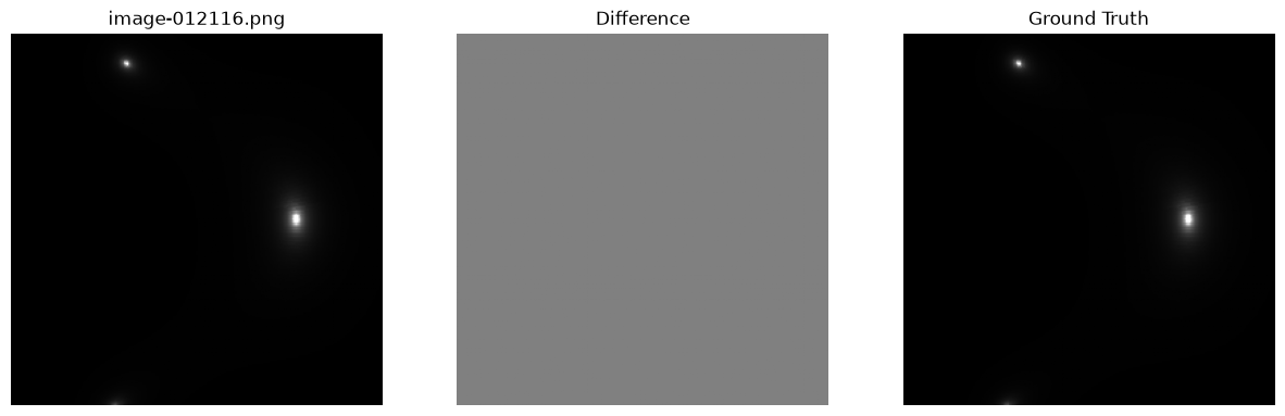
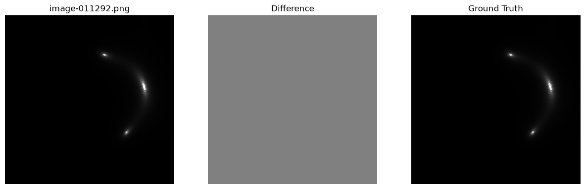
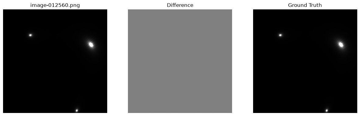
Again, there is no visible discrepancy.

Simulations from Lens Parameters¶

We can also load the original lens parameters, from which the ground truth was computed.

orig = pd.read_csv( "../sie-dataset.csv", index_col="filename" )
display( orig.head() )

Loading...

This dataset is different from the others, giving physical parameters of the lens instead of roulette amplitudes in a point of observation. Thus, we need a different simulator. On a positive note, we can use raytrace simulation, which is accurate.

The SimImage simulator is parameterised in a slightly different way. We need to add the row data from the dataset to the Parameters object instead of passing it as a separate argument. To avoid interference, we make a new Parameters object for the raytrace simulation.

cfg["simulator"]["model"] = "Raytrace"
cfg["simulator"]["centred"] = True
cfg["lens"] = { "mode" : "SIE" }
p2 = cs.Parameters( cfg )
from pprint import pprint
pprint( cfg )

{'lens': {'mode': 'SIE'},
 'simulator': {'centred': True,
               'cropsize': 256,
               'imagesize': 512,
               'model': 'Raytrace',
               'nterms': 4,
               'xireference': True},
 'source': {'mode': 'SersicSphere'}}

We can review these parameters and make sure that they match the original param when it should.

for fn in worst:
    dfsim = rg.Resim(df.loc[fn],param=param,verbose=0)
    dfim = dfsim.getImage()
    p2.setRow( orig.loc[fn] )
    gtsim = dg.SimImage(param=p2,verbose=0)
    gtim = gtsim.getImage()
    csimg.imageCompare( dfim, gtim, 
                        fn, "Original raytrace simulation", 
                        axiscross=True )
    plt.savefig( f"lens-{fn}" )

[getSource] src=SersicSphere, ltprf0=None, verbose=1
[SphericalSource] constructor done

[getSource] src=SersicSphere, ltprf0=None, verbose=1
[SphericalSource] constructor done

[getSource] src=SersicSphere, ltprf0=None, verbose=1
[SphericalSource] constructor done

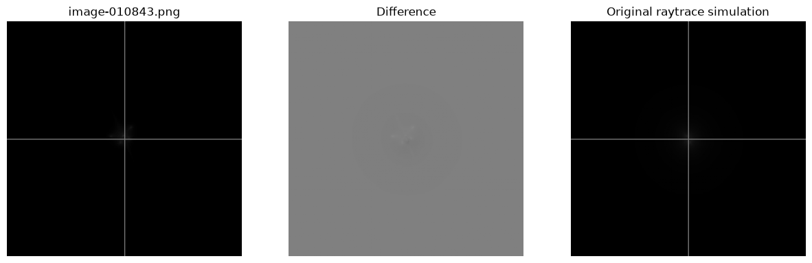
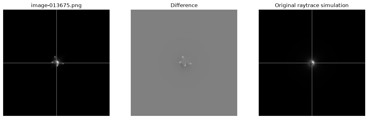
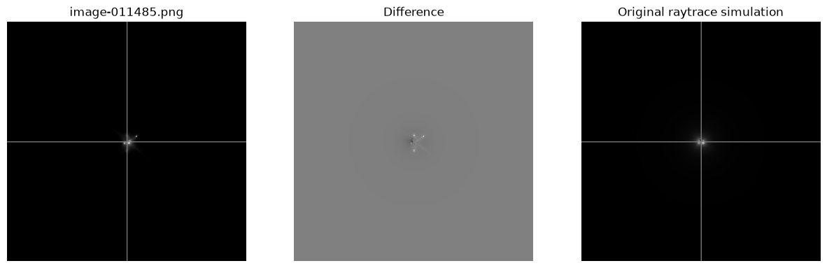
The match is not perfect, but we do see that the primary image is correctly placed. The shape is not accurate on the edges. It is significant that the shadow in the difference image around the primary image is either black or white, never both. This means that the image is smaller or larger, and not rotated or awfully misshaped in general. Clearly, this is a limitation of the roulette formalism, since there is no difference between reconstructed and ground truth simulation.

for fn in best:
    dfsim = rg.Resim(df.loc[fn],param=param,verbose=0)
    dfim = dfsim.getImage()
    p2.setRow( orig.loc[fn] )
    gtsim = dg.SimImage(param=p2,verbose=0)
    gtim = gtsim.getImage()
    csimg.imageCompare( dfim, gtim, fn, "Original raytrace simulation", axiscross=True )
    plt.savefig( f"lens-{fn}" )

[getSource] src=SersicSphere, ltprf0=None, verbose=1
[SphericalSource] constructor done

[getSource] src=SersicSphere, ltprf0=None, verbose=1
[SphericalSource] constructor done

[getSource] src=SersicSphere, ltprf0=None, verbose=1
[SphericalSource] constructor done

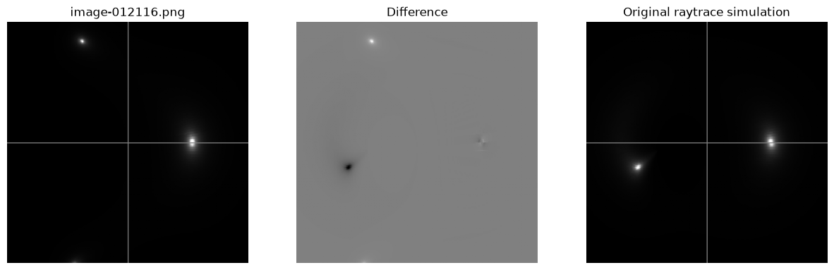
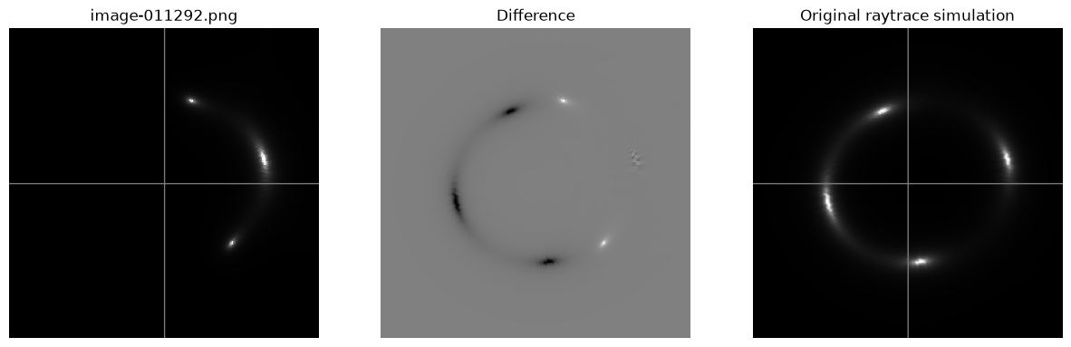
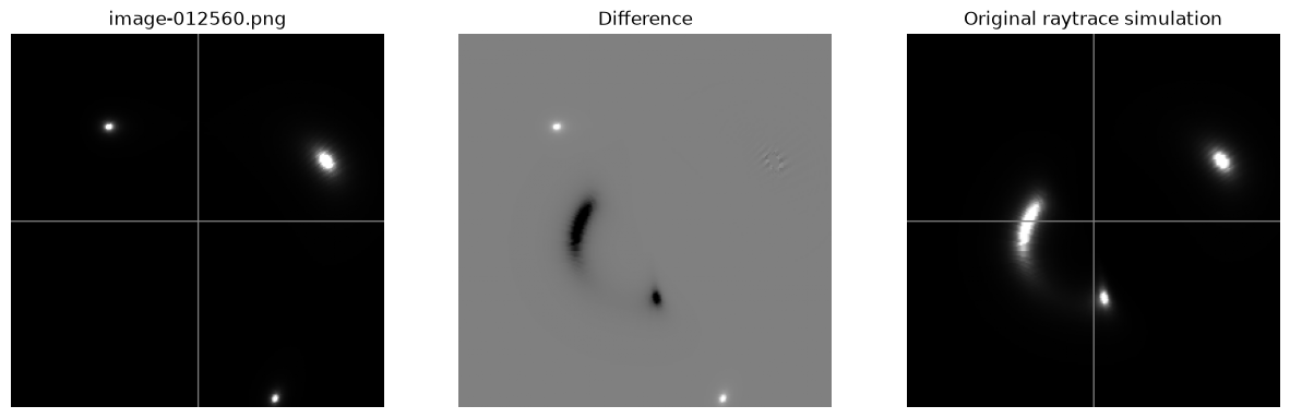
The match to raytrace simulations is not perfect. There is some numerical error around the primary image, although this may be invisible at low screen resolution.

This kind of minor discrepancy is often caused by image post-processing, and may conceivable, in this case, be caused by the centring of the image. We will test this hypothesis in Roulette Resimulation (Experiment July 2026).

We see that the best images display a lot more visible light.

Using the roulette file¶

We redefine gt from the original roulette CSV file and rerun the last experiment.

gt = pd.read_csv( "../sie-roulette.csv", index_col="filename" )

This dataset is different from the others, giving physical parameters of the lens instead of roulette amplitudes in a point of observation. Thus, we need a different simulator. On a positive note, we can use raytrace simulation, which is accurate.

The SimImage simulator is parameterised in a slightly different way. We need to add the row data from the dataset to the Parameters object instead of passing it as a separate argument. To avoid interference, we make a copy of params.

cfg["simulator"]["model"] = "Raytrace"
cfg["simulator"]["centred"] = True
cfg["lens"] = { "mode" : "SIE" }
p2 = cs.Parameters( cfg )
from pprint import pprint
pprint( cfg )

{'lens': {'mode': 'SIE'},
 'simulator': {'centred': True,
               'cropsize': 256,
               'imagesize': 512,
               'model': 'Raytrace',
               'nterms': 4,
               'xireference': True},
 'source': {'mode': 'SersicSphere'}}

for fn in worst:
    dfsim = rg.Resim(df.loc[fn],param=param,verbose=0)
    dfim = dfsim.getImage()
    p2.setRow( orig.loc[fn] )
    gtsim = dg.SimImage(param=p2,verbose=0)
    gtim = gtsim.getImage()
    csimg.imageCompare( dfim, gtim, 
                        fn, "Original raytrace simulation", 
                        axiscross=True )
    plt.savefig( f"file-{fn}" )

[getSource] src=SersicSphere, ltprf0=None, verbose=1
[SphericalSource] constructor done

[getSource] src=SersicSphere, ltprf0=None, verbose=1
[SphericalSource] constructor done

[getSource] src=SersicSphere, ltprf0=None, verbose=1
[SphericalSource] constructor done

The match is not perfect, but we do see that the primary image is correctly placed. The shape is not accurate on the edges. It is significant that the shadow in the difference image around the primary image is either black or white, never both. This means that the image is smaller or larger, and not rotated or awfully misshaped in general. Clearly, this is a limitation of the roulette formalism, since there is no difference between reconstructed and ground truth simulation.

for fn in best:
    dfsim = rg.Resim(df.loc[fn],param=param,verbose=0)
    dfim = dfsim.getImage()
    p2.setRow( orig.loc[fn] )
    gtsim = dg.SimImage(param=p2,verbose=0)
    gtim = gtsim.getImage()
    csimg.imageCompare( dfim, gtim, fn, "Original raytrace simulation", axiscross=True )
    plt.savefig( f"file-{fn}" )

[getSource] src=SersicSphere, ltprf0=None, verbose=1
[SphericalSource] constructor done

[getSource] src=SersicSphere, ltprf0=None, verbose=1
[SphericalSource] constructor done

[getSource] src=SersicSphere, ltprf0=None, verbose=1
[SphericalSource] constructor done

Interestingly, the best images do not perform any better than the worst in terms of visual comparison between roulettes and raytrace.

Conclusion¶

We see that this machine learning model make accurate prediction as far as optical perception goes, but there are limitations to the roulette representations.

This means that there is nothing to gain from further research on machine learning models at this stage.

Abstract¶

Configuration¶

Model evaluation¶

Object evaluation¶

Simulation from Roulette Amplitudes¶

Dealing with low contrast images¶

Full image set¶

Simulations from Lens Parameters¶

Using the roulette file¶

Conclusion¶