Abstract
This is work in progress. We are debugging the report format.
This document will investigate inaccuracies in the standard evaluation document, Evaluation of machine learning for SIE. We hypothesised that image centring causes minor numerical inaccuracy, which differs between the original raytrace image and the roulette resimulation.
We build on CosmoSim Demo III Roulette Resimulation. The following modules are needed.
import pandas as pd
import matplotlib.pyplot as plt
import numpy as np
import tomllib as tl

from CosmoSim.datagen import SimImage
import CosmoSim.Image as csimg
from CosmoSim import Parameters
from CosmoSim.roulettegen import Resim

import CosmoSim as cs
print( "CosmoSim version", cs.__version__ )
CosmoSim version 3.3.0
We will also need the following files, which will be loaded by the code:
Review of the SIE experiment data
We load and compare the testing results and the ground truth.
gt = pd.read_csv( "../sie-testing.csv", index_col="filename" )
pr = pd.read_csv( "pred-sie-testing.csv", index_col="filename" )
rawerrors = gt - pr
sse = (rawerrors**2).sum(axis=1)
From the dataset, we pick the three best and the three worst data points.
best = list(sse.nlargest(3).index)
worst = list(sse.nsmallest(3).index)
print( "Best:", best )
print( "Worst:", worst )
Best: ['image-012116.png', 'image-011292.png', 'image-012560.png']
Worst: ['image-010843.png', 'image-013675.png', 'image-011485.png']
Simulation from lens parameters
To simulate the images, we need to load the parameters from
sie-dataset.csv.
From this dataset we pick just the selected rows.
df = pd.read_csv( "../sie-dataset.csv", index_col="filename" )
df = df.loc[best+worst]
display( df.T )We will also need the simulator configuration from sie-dataset.toml.
with open( "../sie-dataset.toml", 'rb' ) as f:
            toml = tl.load(f)
param = Parameters( toml )
Now we can run the simulator.
param.setRow( df.iloc[0] )
param["simulator"]["centred"] = False
raysim0 = SimImage( param.copy(), verbose=0 )
ray0 = raysim0.getImage()
param["simulator"]["model"] = "Roulette"
rousim0 = SimImage( param, verbose=0 )
rou0 = rousim0.getImage()
csimg.imageCompare( ray0, rou0, "Raytrace", "Roulette" ) 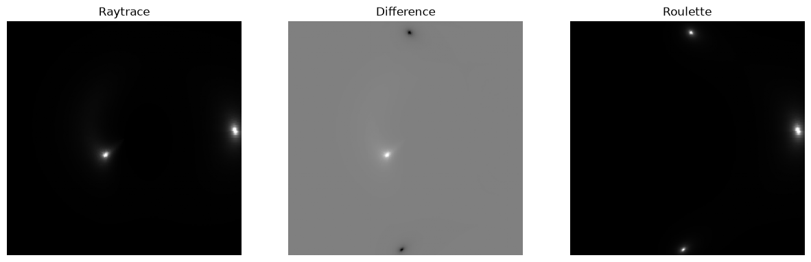
Here we cannot see the discrepancy that we found in Evaluation of machine learning for SIE.
We can also get annotations on the images, like this:
param.setRow( df.iloc[0] )
param["simulator"]["centred"] = False
ray0a = raysim0.getAnnotated(convergenceRing=None,centrePoint=None)
param["simulator"]["model"] = "Roulette"
rou0a = rousim0.getAnnotated(convergenceRing=None,centrePoint=None)
csimg.imageCompare( ray0a, rou0a, "Raytrace", "Roulette" ) 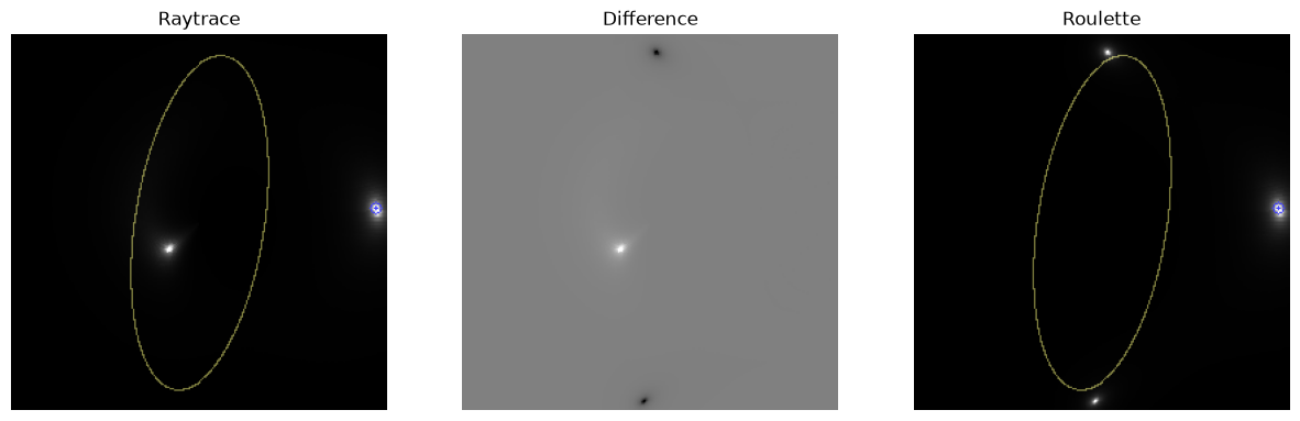
The roulette simulation seems perfect within the convergence ring.
The full image set
We can repeat the simulation on all the selected imags.
for index, row in df.iterrows():
    param.setRow( row )
    param["simulator"]["centred"] = False
    ray = SimImage( param, verbose=0
        ).getAnnotated(centrePoint=None)
    param["simulator"]["model"] = "Roulette"
    rou = SimImage( param, verbose=0
        ).getAnnotated(centrePoint=None)
    csimg.imageCompare( ray, rou, index, "Roulette", axiscross=True )
    plt.savefig( f"annot1-{index}" )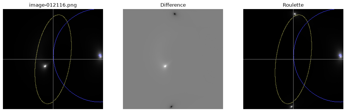
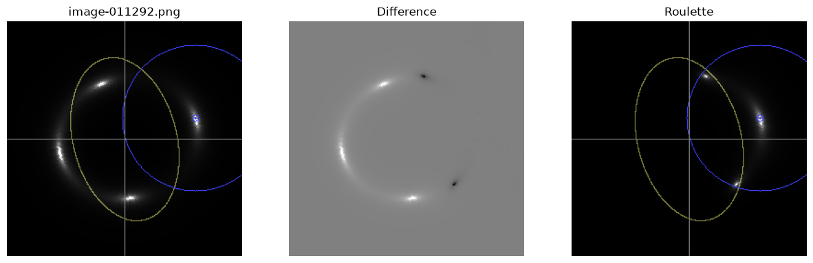
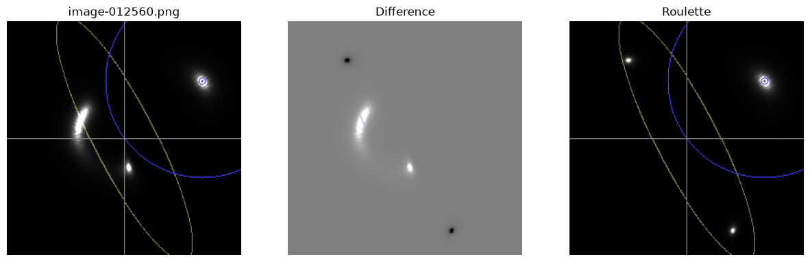
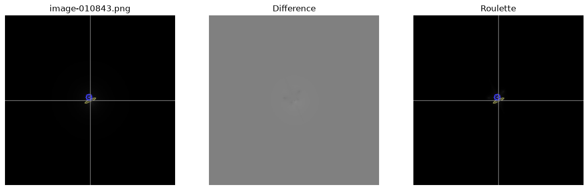
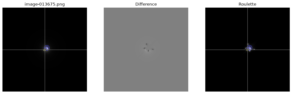
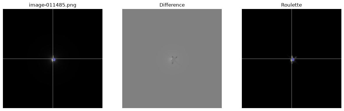
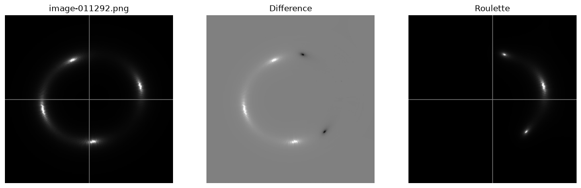
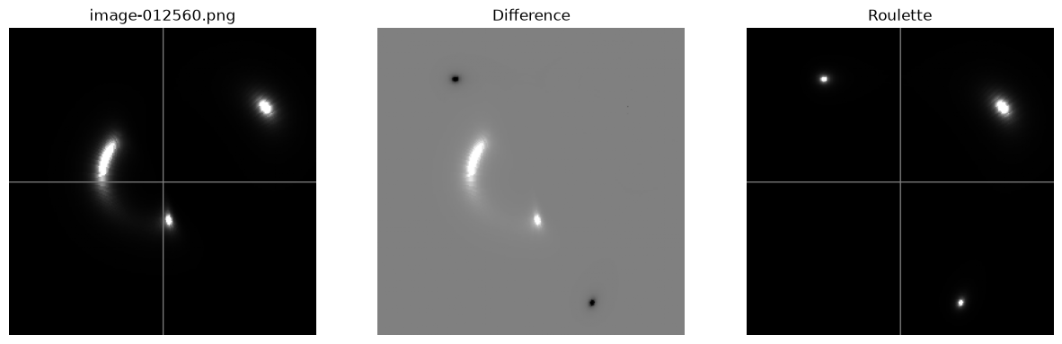
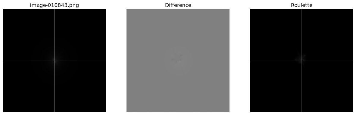
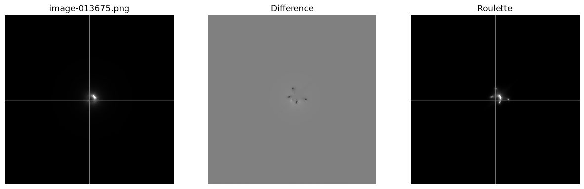
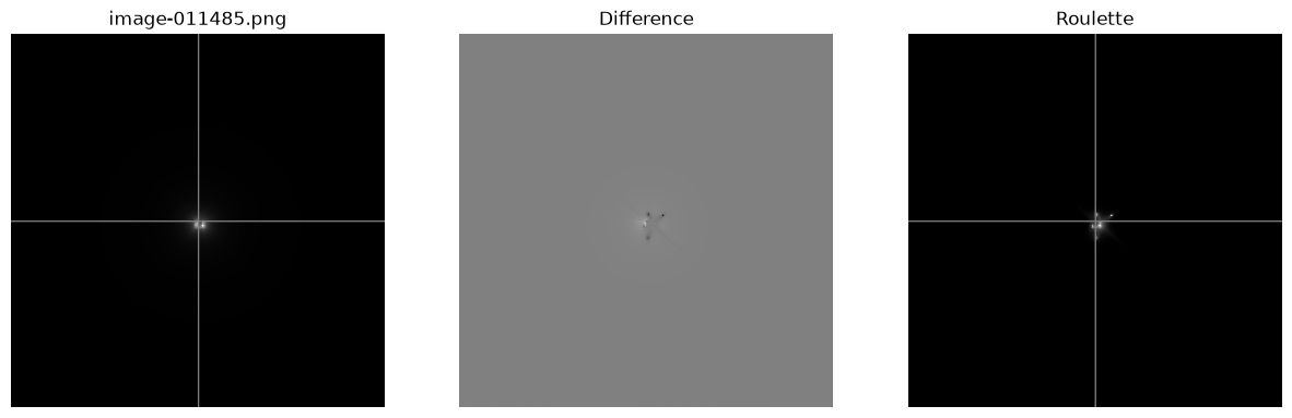
These images show good match between raytrace and roulette, although it may be hard to judge when the visible image is small and close to the origin. Where the primary image is far from the origin, the match looks perfect. It may be somewhat easier to see without the annotations.
for index, row in df.iterrows():
    param.setRow( row )
    param["simulator"]["centred"] = False
    ray = SimImage( param, verbose=0
        ).getImage()
    param["simulator"]["model"] = "Roulette"
    rou = SimImage( param, verbose=0
        ).getImage()
    csimg.imageCompare( ray, rou, index, "Roulette", axiscross=True )
    plt.savefig( f"resim1-{index}" )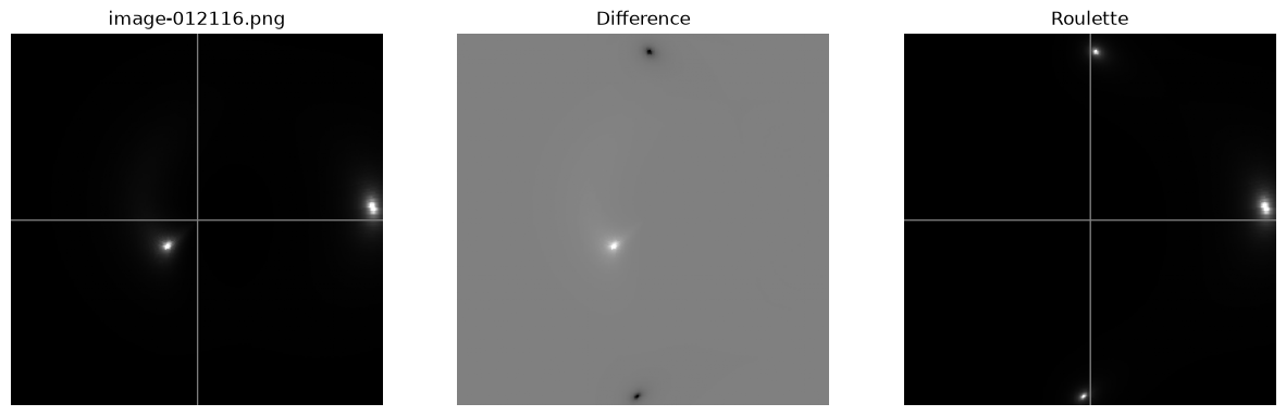
Resimulation
It will be interesting to check if resimulation confirms the result. First a simple check with a single data point.
row = raysim0.getData()
display( row )
filename image-012116.png
source SersicSphere
x 42.9933
y 10.8804
sigma 18.9116
sigma2 34.4593
theta 70.1152
luminosity 73.3291
n_sersic 3.4013
lensX 0
lensY 0
centreX 0
centreY 0
reletaX 42.9933
reletaY 10.8804
offsetX -0.000434
offsetY -78.230844
xiX 119.96727
xiY 9.62396
alpha[0][1] -76.974404
alpha[1][0] -0.189082
alpha[1][2] 0.186664
alpha[2][1] 0.002386
alpha[2][3] -0.002326
alpha[3][0] -0.000019
alpha[3][2] -0.000029
alpha[3][4] 0.000045
alpha[4][1] 0.000001
alpha[4][3] 0.000001
alpha[4][5] -0.000001
beta[0][1] 1.261843
beta[1][0] 0.0
beta[1][2] 0.030143
beta[2][1] -0.000274
beta[2][3] -0.00041
beta[3][0] 0.0
beta[3][2] 0.000006
beta[3][4] 0.00001
beta[4][1] -0.0
beta[4][3] -0.0
beta[4][5] -0.0
Name: image-012116.png, dtype: objectnewcfg = { "simulator" : { "cropsize" : 256, "nterms" : 4, "centred" : False }
, "source" : { "mode" : "SersicSphere" }
}
rp = Parameters( newcfg )
resimImage = Resim( row, rp, verbose=0 ).getImage()
csimg.imageCompare( resimImage, rou0, "Resimulation", "Original Roulette" )
csimg.imageCompare( resimImage, ray0, "Resimulation", "Original Raytrace" )[getSource] src=SersicSphere, ltprf0=None, verbose=1
[SphericalSource] constructor done
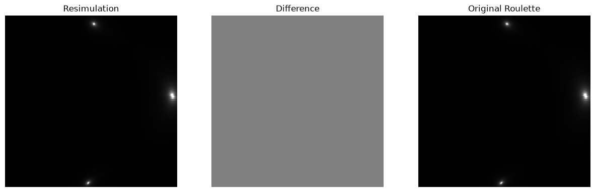
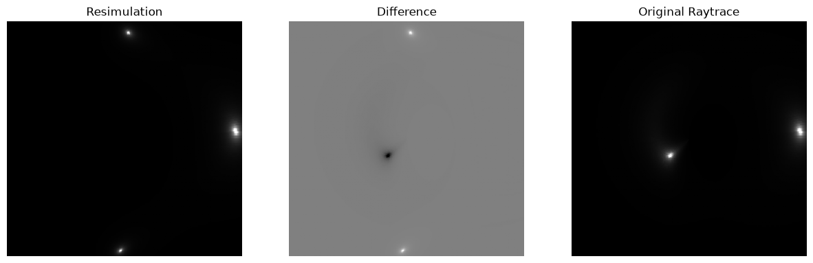
This looks perfect as far as the roulette formalism goes, as do the other selected images.
for index, row in df.iterrows():
param.setRow( row )
param["simulator"]["centred"] = False
imsim = SimImage( param, verbose=0 )
ray = imsim.getImage()
rr = imsim.getData()
rou = Resim( rr, rp, verbose=0 ).getImage()
csimg.imageCompare( ray, rou, "Raytrace", "Roulette", axiscross=True )
plt.savefig( f"resim2-{index}" )[getSource] src=SersicSphere, ltprf0=None, verbose=1
[SphericalSource] constructor done
[getSource] src=SersicSphere, ltprf0=None, verbose=1
[SphericalSource] constructor done
[getSource] src=SersicSphere, ltprf0=None, verbose=1
[SphericalSource] constructor done
[getSource] src=SersicSphere, ltprf0=None, verbose=1
[SphericalSource] constructor done
[getSource] src=SersicSphere, ltprf0=None, verbose=1
[SphericalSource] constructor done
[getSource] src=SersicSphere, ltprf0=None, verbose=1
[SphericalSource] constructor done
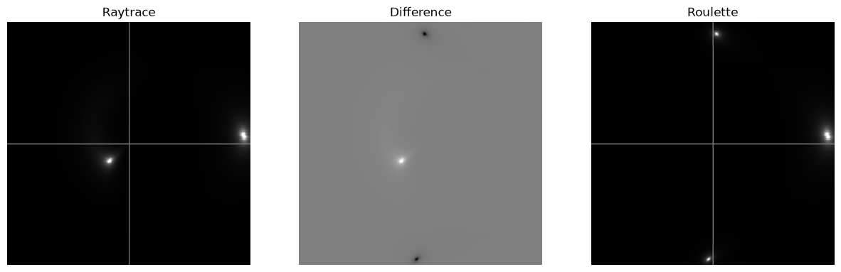
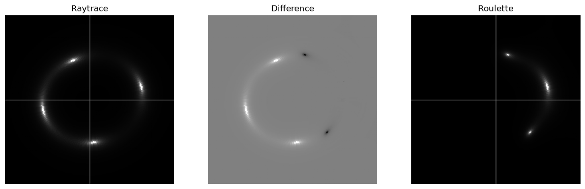
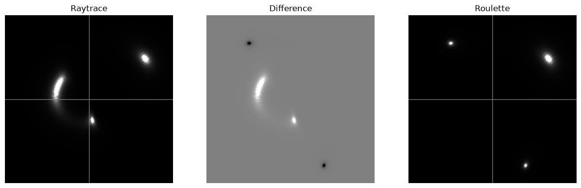
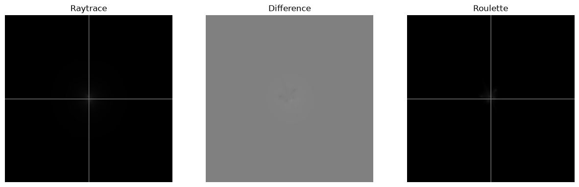
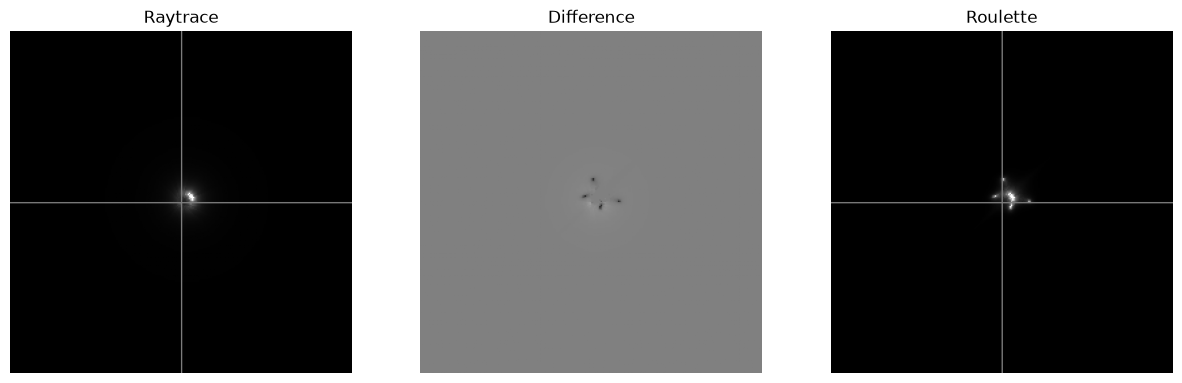
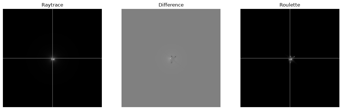
Note that we have simulated without centring.
print( "Centring:", param.get( "centred" ) )Centring: False
Centred mode
Let us reset the simulator to use centred mode. Here we will see the numeric inaccuracy.
with open( "../sie-dataset.toml", 'rb' ) as f:
toml = tl.load(f)
param = Parameters( toml )for index, row in df.iterrows():
param.setRow( row )
imsim = SimImage( param, verbose=0 )
ray = imsim.getImage()
rr = imsim.getData()
rou = Resim( rr, rp, verbose=0 ).getImage()
csimg.imageCompare( ray, rou, index, "Roulette", axiscross=True )
plt.savefig( f"centre-{index}" )[getSource] src=SersicSphere, ltprf0=None, verbose=1
[SphericalSource] constructor done
[getSource] src=SersicSphere, ltprf0=None, verbose=1
[SphericalSource] constructor done
[getSource] src=SersicSphere, ltprf0=None, verbose=1
[SphericalSource] constructor done
[getSource] src=SersicSphere, ltprf0=None, verbose=1
[SphericalSource] constructor done
[getSource] src=SersicSphere, ltprf0=None, verbose=1
[SphericalSource] constructor done
[getSource] src=SersicSphere, ltprf0=None, verbose=1
[SphericalSource] constructor done
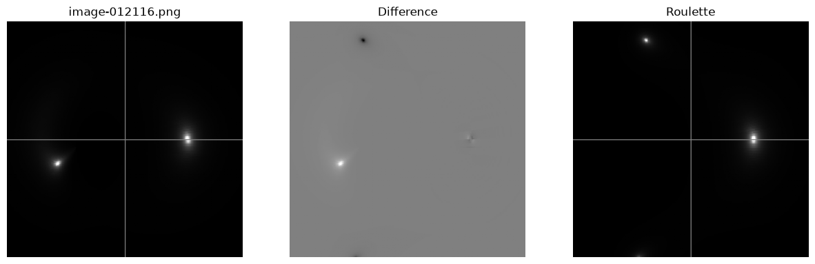
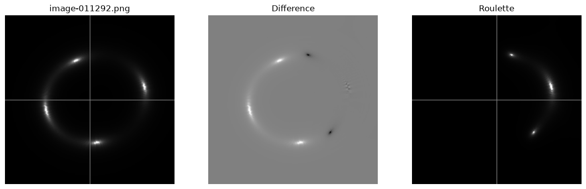
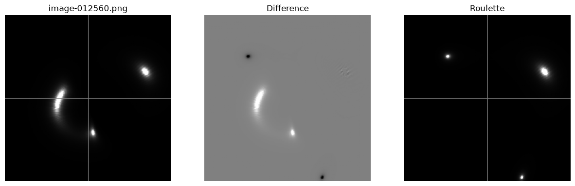
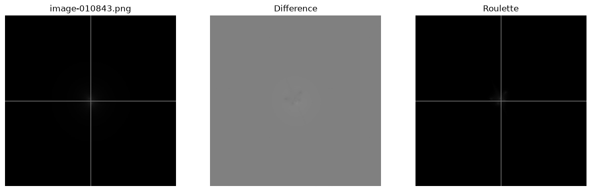
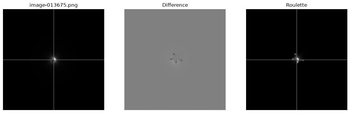
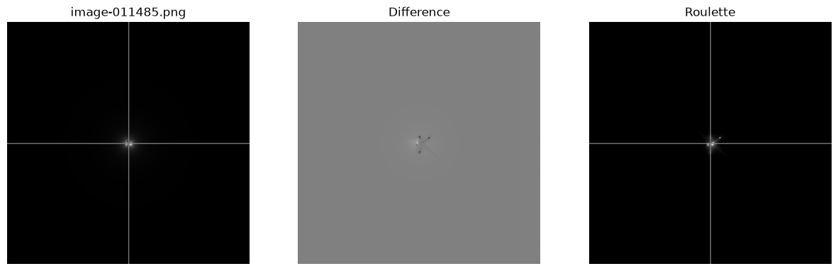
This is also perfect.
Validation of the generated amplitudes
During the debugging phase, we also check the amplitudes generated here against the file generated by the batch run. Although this did not give any answers at the time, we give the code in case it may be useful in the future.
gt = pd.read_csv( "../sie-roulette.csv", index_col="filename" )
gt = gt.loc[best+worst]
display( gt )We did not store the amplitudes from getData when we did the simulation, so we need to create a DataFrame of these amplitudes now.
l = []
for index, row in df.iterrows():
    param.setRow( row )
    imsim = SimImage( param, verbose=0 )
    l.append( imsim.getData() )
gen = pd.DataFrame( l )
display( gen )The interesting step is now to compare gen to the ground truth gt.
diff = gen.drop("source",axis=1)-gt
display( diff )This looks like a good match, but to make sure we do not miss anything, we can look at the maximum absolute differences.
display( diff.abs().max() )alpha[0][1] 4.440892e-16
alpha[1][0] 8.326673e-17
alpha[1][2] 6.938894e-17
alpha[2][1] 8.673617e-17
alpha[2][3] 8.066464e-17
alpha[3][0] 9.714451e-17
alpha[3][2] 9.714451e-17
alpha[3][4] 1.908196e-17
alpha[4][1] 6.938894e-17
alpha[4][3] 3.989864e-17
alpha[4][5] 9.801188e-17
beta[0][1] 2.220446e-16
beta[1][0] 0.000000e+00
beta[1][2] 8.326673e-17
beta[2][1] 6.938894e-17
beta[2][3] 9.540979e-17
beta[3][0] 0.000000e+00
beta[3][2] 9.714451e-17
beta[3][4] 7.632783e-17
beta[4][1] 6.863000e-17
beta[4][3] 9.324139e-17
beta[4][5] 8.586881e-17
centreX 5.551115e-17
centreY 0.000000e+00
filename NaN
lensX 5.551115e-17
lensY 0.000000e+00
luminosity 0.000000e+00
n_sersic 0.000000e+00
offsetX 9.454243e-17
offsetY 5.551115e-17
reletaX 0.000000e+00
reletaY 8.326673e-17
sigma 0.000000e+00
sigma2 0.000000e+00
source NaN
theta 0.000000e+00
x 0.000000e+00
xiX 0.000000e+00
xiY 3.552714e-15
y 0.000000e+00
dtype: float64Right, so differences are around 10-14 and smaller.
Closure
This comparison shows good match between raytrace and roulette, except possibly for small images close to the origin. It also demonstrates that the new mode of operation in v3.3 is a necessary improvement.
Using roulette resimulation to validate machine learning predictions, we have to expect a numeric inaccuracy, due to the centring of the images subjected to the machine learning model. This is probably not a problem in practice, since observational images will show all sorts of inaccuracies in any event.