CosmoSim Demo III Roulette Resimulation

This Demo assumes that you are familiar with the principles from Demo01.md. We start with the same imports

import pandas as pd
import matplotlib.pyplot as plt
import numpy as np
from PIL import Image
import tomllib as tl

from CosmoSim.datagen import SimImage
import CosmoSim.Image as csimg
from CosmoSim import Parameters

import CosmoSim as cs
print( "CosmoSim version", cs.__version__ )

CosmoSim version 3.2.2b2

Additionally, we require the Resim class for resimulation.

from CosmoSim.roulettegen import Resim

The Resim class shares the GenericSim superclass with SimImage, which we used in Demo01.md but simulates from precomputed roulette parameters and not from a regular lens model.

Basic Configuration¶

We start with parameters similar to the ones from Demo01.md, to make a baseline raytrace simulation using a SIE lens. We have just rounded some of the parameters to get neater numbers. We will use the simulation from SimImage to get roulette amplitudes for resimulation.

with open( "Demo03.toml", 'rb' ) as f:
            toml = tl.load(f)

param = Parameters( toml )
imsim = SimImage( param, verbose=0 )
im = imsim.getImage()
csimg.imshow( im, "Baseline simulation" )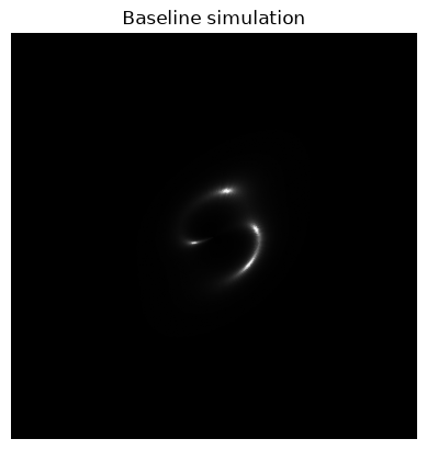

Tip

For debugging, it may be useful to change the verbosity level on the fly. On this point, the C++ code functions differently from the python code. Where the python code often has per-class and per-function verbosity settings, the C++ code uses a single global variable which can be set thus:

from CosmoSim.CosmoSimPy import setDebug
setDebug(3)

This is set every time the Resim or SimImage classes are instantiated, which works well enough if only one instance is made, or all use the same verbosity level. For more complex situations, the above setDebug may be useful. We used it during debugging, but it has now been from the final demo.

Roulette parameters¶

We can retrieve the roulette amplitudes with the getData() method. The resulting data is a pandas Series.

row = imsim.getData()
display( row )

filename              test.png
source         SersicEllipsoid
x                           12
y                            6
sigma                       10
sigma2                      30
theta                       45
lensX                        0
lensY                        0
centreX                      0
centreY                      0
reletaX                   12.0
reletaY                    6.0
offsetX                   -0.0
offsetY              -22.36068
xiX                   56.72136
xiY                   28.36068
alpha[0][1]                0.0
alpha[1][0]           -0.39422
alpha[1][2]           0.236532
alpha[2][1]            0.00834
alpha[2][3]          -0.001668
alpha[3][0]          -0.000074
alpha[3][2]          -0.000176
alpha[3][4]          -0.000103
alpha[4][1]           0.000005
alpha[4][3]           0.000003
alpha[4][5]           0.000014
alpha[5][0]               -0.0
alpha[5][2]               -0.0
alpha[5][4]                0.0
alpha[5][6]          -0.000001
beta[0][1]                 0.0
beta[1][0]                 0.0
beta[1][2]            0.315376
beta[2][1]             0.00417
beta[2][3]           -0.009174
beta[3][0]                 0.0
beta[3][2]           -0.000235
beta[3][4]            0.000353
beta[4][1]            0.000003
beta[4][3]            0.000014
beta[4][5]           -0.000015
beta[5][0]                 0.0
beta[5][2]                -0.0
beta[5][4]           -0.000001
beta[5][6]            0.000001
Name: test.png, dtype: object

Here we see that we have roulette amplitudes up to order 5, which is the maximum implemented for analytical SIE.

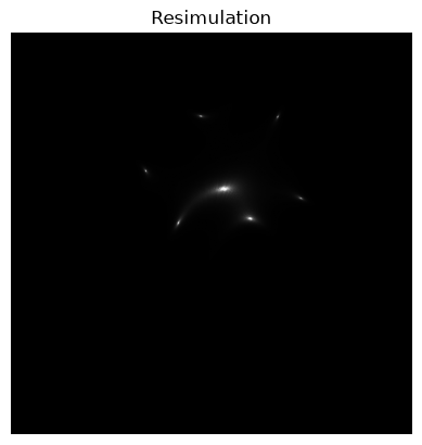
rsim = Resim( row )
resimImage = rsim.getImage()
csimg.imshow( resimImage, "Resimulation" )

[loadData] deducing nterms = None
xi 56.72135954999579 28.360679774997894 10
Initialised simulator at point (0, 0)
[getSource] src=SersicEllipsoid, ltprf0=None, verbose=1
[getSource] mode=SourceSpec.Ellipse, ltprf=LightProfileSpec.Sersic
Instantiating RouletteModel ... 
[SimulatorModel::setNterms] 10 -> 5
[setNu] etaOffset set to zero.
[RouletteRegenerator::setCentre] etaOffset = [0, 0]; nu=[0, 0]; eta=[0, 0]; xi=[0, 0]
[EllipsoidSource ] sz=512; sigma1=10; sigma2=30; theta=0.785398; lightprf=0
[SimulatorModel::setSource] setting source
[RouletteRegenerator] updateApparentAbs() does nothing.
[SimulatorModel::update] Done updateApparentAbs()
[SimulatorModel::update] thread section
[Source::getImage()]
[SimulatorModel::updateInner()] eta=[0, 0]
[calculateAlphaBeta] No lens - does nothing.
[SimulatorModel::parallelDistort] 4 threads (maskMode=0)
[SimulatorModel::parallelDistort] etaOffset=[0, 0]; nu=[0, 0]; eta[0, 0]; referenceXi=[0, 0]
[SimulatorModel] No mask 
[SimulatorModel::parallelDistort] lower=0; rng=512; rng1=128
Time to update(): 73 milliseconds
[Simulator] Centre Point (-4.00,-1.73) (Centre of Luminence in Planar Co-ordinates)
[getImage] centring from parameters: None

For reference, we can do the original roulette simulation, using a SimImage object.

param["simulator"]["model"] = "Roulette"
roulette = SimImage( param, verbose=0 )
rouletteImage = roulette.getImage()
csimg.imshow( rouletteImage, "Roulette simulation" )

[SimulatorModel::getDistorted()]
[setDebug] 0

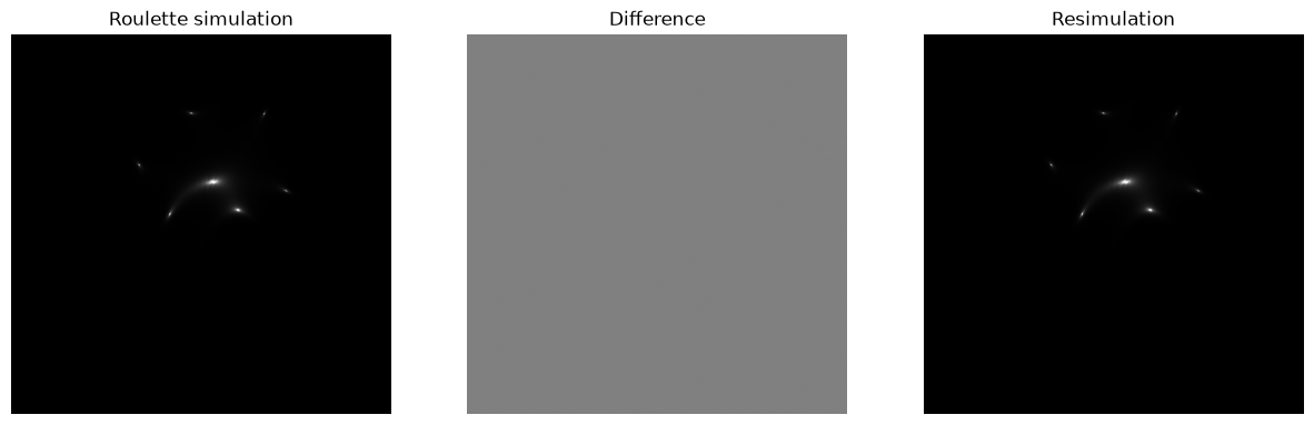
The two roulette simulations look similar but displaced compared to each other.

The Source¶

We can also have a look at the original source image.

actual = rsim.getActualImage()
csimg.imshow( actual, "Actual source image" )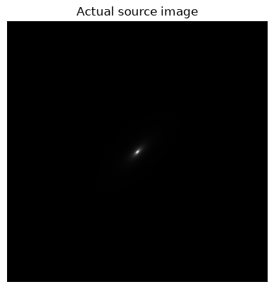

actual image <class 'numpy.ndarray'>

Comparison¶

To compare the images, we can plot side by side We also add reference lines to each image, except the difference image. If the code is confusing, it is because we

imdiff = csimg.imageDiff(rouletteImage,resimImage)
rdiff = csimg.imageDiff(rouletteImage,im)

csimg.drawAxes(actual)
csimg.drawAxes(im)
csimg.drawAxes(rouletteImage)
csimg.drawAxes(resimImage)

fig = plt.figure(figsize=(15,10))
fig.tight_layout(pad=0.0)
plt.subplots_adjust(hspace=0.1, wspace=0.1) 

fig.add_subplot(2, 3, 1)
csimg.imshow( actual, "Actual source image" )
fig.add_subplot(2, 3, 2)
csimg.imshow( im, "Original raytrace simulation" )
fig.add_subplot(2, 3, 3)
csimg.imshow( rdiff, "Roulette/raytrace difference" )
fig.add_subplot(2, 3, 5)
csimg.imshow( imdiff, "Difference image" )
fig.add_subplot(2, 3, 4)
csimg.imshow( rouletteImage, "Roulette simulation" )
fig.add_subplot(2, 3, 6)
csimg.imshow( resimImage, "Resimulation" )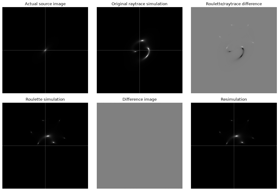

Centring the image¶

In the original simulation, centring is straight forward, by setting simulator.centred to True.

param["simulator"]["centred"] = True
param["simulator"]["model"] = "Raytrace"
imsim = SimImage( param, verbose=0 )
imC = imsim.getImage(verbose=1)

fig = plt.figure(figsize=(10,5))
fig.tight_layout(pad=0.0)
plt.subplots_adjust(hspace=0.1, wspace=0.1) 

fig.add_subplot(1, 2, 1)
csimg.imshow( imC, "Original simulation - centred" )
fig.add_subplot(1, 2, 2)
csimg.imshow( csimg.imageDiff(imC,im), "Difference" )

[getImage] centring from parameters: True

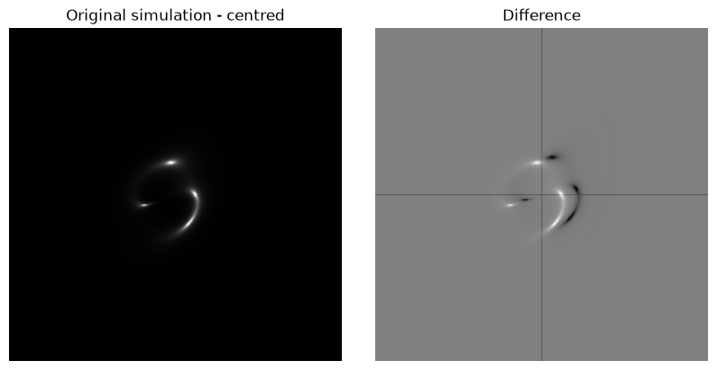
We have plotted the difference image to see that centring does make a difference. We can also note the difference it makes to the data for resimulation.

rowC = imsim.getData()
display( pd.DataFrame( [row, rowC] ).transpose() )

Loading...

The roulette amplitudes do not change. The are calculated in the same point. However the relative source position reletaX/reletaY does. It is the sum of the original position and the centrepoint centreX/centreY.

We can do the same with roulette; centred is still True.

param["simulator"]["model"] = "Roulette"
roulette = SimImage( param, verbose=0 )
rouletteImageC = roulette.getImage(verbose=0)

fig = plt.figure(figsize=(10,5))
fig.tight_layout(pad=0.0)
plt.subplots_adjust(hspace=0.1, wspace=0.1) 

fig.add_subplot(1, 2, 1)
csimg.imshow( rouletteImageC, "Roulette simulation - centred" )
fig.add_subplot(1, 2, 2)
csimg.imshow( csimg.imageDiff(rouletteImageC,rouletteImage), "Difference" )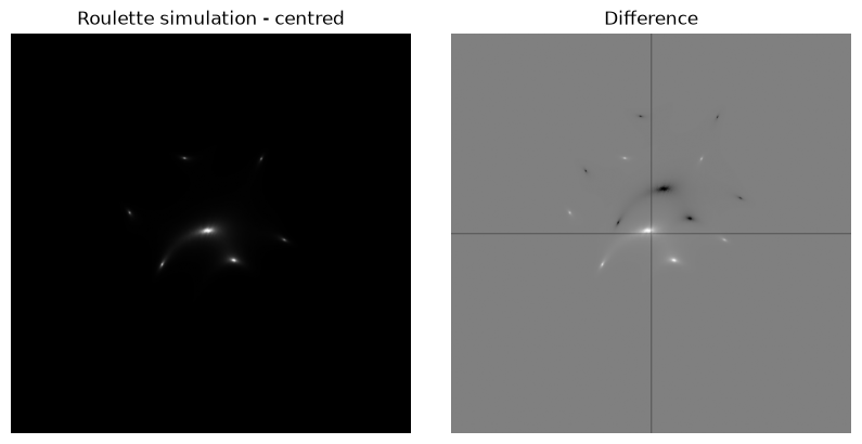

Finally we resimulate from the data from the centred simulatior. We compare the result with both the original resimulation and with the centred raytrace.

rsim = Resim( rowC, verbose=0 )
resimImageC = rsim.getImage()

fig = plt.figure(figsize=(15,5))
fig.tight_layout(pad=0.0)
plt.subplots_adjust(hspace=0.1, wspace=0.1) 

fig.add_subplot(1, 3, 1)
csimg.imshow( resimImageC, "Resimulation from centred image" )
fig.add_subplot(1, 3, 2)
csimg.imshow( csimg.imageDiff(resimImageC,resimImage), "Difference with previous resimulation" )
fig.add_subplot(1, 3, 3)
csimg.imshow( csimg.imageDiff(resimImageC,imC), "Difference with centred raytrace" )

[getSource] src=SersicEllipsoid, ltprf0=None, verbose=1
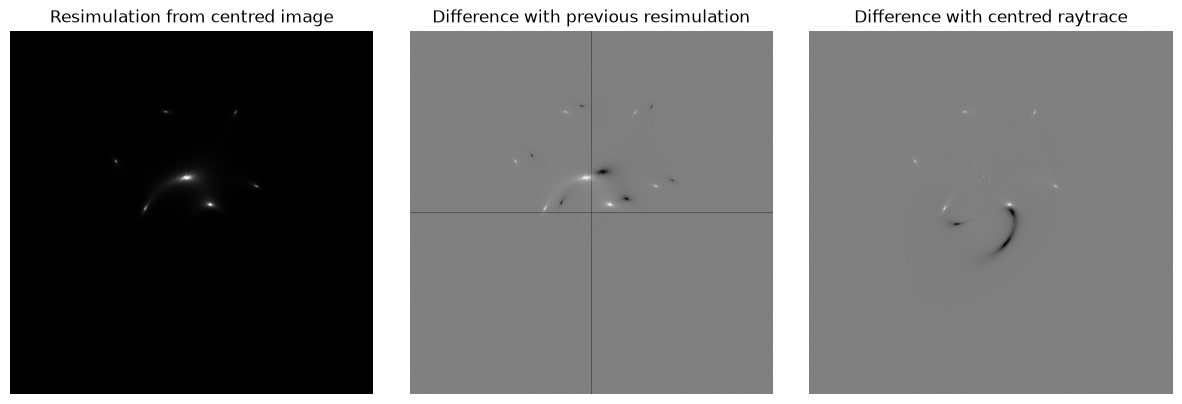
[getSource] mode=SourceSpec.Ellipse, ltprf=LightProfileSpec.Sersic

We note that the image has shifted compared to the original resimulation.
The right hand image shows that the co-ordinate system is shifted to match the centred raytrace image.

Closure¶

Resmulation is going to be critical to evaluate machine learning models in practical scenarioes. The resimulated image can be compared to the observation without having a ground truth for the roulette amplitudes.

There is some work in progress here.
I hope we have managed to demonstrate some of the caveats, particularly with respect to centring. Documentation of Implementation and the definitions of the different co-ordinate systems is ongoing work.