CosmoSim Demo I - CosmoSim

Preparation¶

We will use pandas to handle sets of lensing systems with different parameters, pyplot for plotting, PIL for images, as well as config files in TOML. Hence we import the following modules.

import pandas as pd
import matplotlib.pyplot as plt
import numpy as np
from PIL import Image
import toml, json

From CosmoSim, we will use the main simulator CosmoSim and the data generator datagen.

from CosmoSim.datagen import SimImage
import CosmoSim.Image as csimg
from CosmoSim import Parameters

Given that CosmoSim is under continued development, it is useful to check the version.

from CosmoSim import __version__
print( "CosmoSim version", __version__ )

CosmoSim version 3.2.3

Simulating an image¶

In this demo, we will use the following sample parameters, taken from a test by Ben David 6 May 2026. CosmoSim can take parameters in many different formats. CSV files are generally used for bulk processing, while TOML is more convenient for individual samples. The notation is not always harmonised, and is shown here for reference.

GUI Name	Parameter	CSV name	TOML Name
Einstein Radius	$R_E= 46$	`einsteinradius`	`lens.einsteinR`
Ellipticity	0.34	`ellipseratio`	`lens.ellipseratio`
Lens Orientation	107	`orientation`	`lens.orientation`
Distance Ratio (chi)	$\chi=50\%$	`chi`	`lens.chi`
x	$x= 11.01$	`x`	`position.x`
y	$y= 0.31$	`x`	`position.y`
Source Size	$\sigma=20$	`sigma`	`source.sigma`
Source Rotation	45°	`theta`	`source.theta`

First test of the API¶

We can define the configuration as a dict using the nested (TOML) structure.

cfg = { 'lens': { 
            'einsteinradius': 46,
            'ellipseratio': 0.34,
            'orientation': 107 }
      , 'source': {
            'mode': 'Spherical',
            'sigma': 20,
            'position': 'cartesian'}
      , 'position': {'x': 11.01, 'y': 0.31}
      }

CosmoSim uses Parameters objects which store the parameters as a cascaded dictionary, incorporating defaults. This is instantiated using the dict that we just made.

param = Parameters( cfg )
print( param )

<{'lens': <{}, Ancestor: <{'einsteinradius': 46, 'ellipseratio': 0.34, 'orientation': 107}, Ancestor: <{}, Ancestor: <{'mode': 'SIS', 'einsteinradius': 20, 'ellipseratio': 0.6, 'orientation': 45}, Ancestor: None>>>>, 'source': <{}, Ancestor: <{'mode': 'Spherical', 'sigma': 20, 'position': 'cartesian'}, Ancestor: <{}, Ancestor: <{'sigma': 10, 'sigma2': 20, 'theta': 45}, Ancestor: None>>>>, 'position': <{}, Ancestor: <{}, Ancestor: <{'x': 11.01, 'y': 0.31}, Ancestor: None>>>, 'simulator': <{}, Ancestor: <{}, Ancestor: <{}, Ancestor: <{'imagesize': 512, 'model': 'Raytrace'}, Ancestor: None>>>>, 'dataset': <{}, Ancestor: None>, 'annotation': <{}, Ancestor: None>, 'management': <{}, Ancestor: <{}, Ancestor: <{}, Ancestor: <{'maxcount': None, 'filename': 'test.png'}, Ancestor: None>>>>}, Ancestor: <{'lens': <{'einsteinradius': 46, 'ellipseratio': 0.34, 'orientation': 107}, Ancestor: <{}, Ancestor: <{'mode': 'SIS', 'einsteinradius': 20, 'ellipseratio': 0.6, 'orientation': 45}, Ancestor: None>>>, 'source': <{'mode': 'Spherical', 'sigma': 20, 'position': 'cartesian'}, Ancestor: <{}, Ancestor: <{'sigma': 10, 'sigma2': 20, 'theta': 45}, Ancestor: None>>>, 'position': <{}, Ancestor: <{'x': 11.01, 'y': 0.31}, Ancestor: None>>, 'simulator': <{}, Ancestor: <{}, Ancestor: <{'imagesize': 512, 'model': 'Raytrace'}, Ancestor: None>>>, 'dataset': <{}, Ancestor: None>, 'annotation': <{}, Ancestor: None>, 'management': <{}, Ancestor: <{}, Ancestor: <{'maxcount': None, 'filename': 'test.png'}, Ancestor: None>>>}, Ancestor: <{'simulator': <{}, Ancestor: <{'imagesize': 512, 'model': 'Raytrace'}, Ancestor: None>>, 'source': <{}, Ancestor: <{'sigma': 10, 'sigma2': 20, 'theta': 45}, Ancestor: None>>, 'lens': <{}, Ancestor: <{'mode': 'SIS', 'einsteinradius': 20, 'ellipseratio': 0.6, 'orientation': 45}, Ancestor: None>>, 'dataset': <{}, Ancestor: None>, 'annotation': <{}, Ancestor: None>, 'management': <{}, Ancestor: <{'maxcount': None, 'filename': 'test.png'}, Ancestor: None>>}, Ancestor: None>>>

We can simulate the configuration by merely instantiating a SimImage object, as follows. The simulator runs as part of the instantiation.
It is rather verbose, with debug messages still left in.

imsim = SimImage( param )

[SimImage] init (verbose=1) ...
[getSource] src=Spherical, ltprf0=None, verbose=1
[getSource] mode=SourceSpec.Sphere, ltprf=LightProfileSpec.Gaussian
[SphericalSource] constructor done
setFile /home/runner/.local/lib/python3.14/site-packages/CosmoSim/sis50.txt
[PsiFunctionLens.initAlphasBetas] Amplitudes file /home/runner/.local/lib/python3.14/site-packages/CosmoSim/sis50.txt
[initAlphasBetas] opened file /home/runner/.local/lib/python3.14/site-packages/CosmoSim/sis50.txt
[SimulatorMode::setLens] SIS
[SimulatorModel::setSource] setting source
[SimulatorModel::setNterms] 10 -> 5
[SimulatorModel::update] Lens: SIS
[SIS::getXi] [11.01, 0.31] -> [56.9918, 1.60467]
[setNu] etaOffset set to zero.
[SimulatorModel::update] Done updateApparentAbs()
[SimulatorModel::update] thread section
[Source::getImage()]
[SimulatorModel::updateInner()] eta=[11.01, 0.31]
[calculateAlphaBeta] [[56.9918, 1.60467]] ... 
[PsiFunctionLens.calculateAlphaBeta()] 5; 46 - [56.9918, 1.60467]
[RaytraceModel] distort() SIS (Spherical Source)
[RaytraceModel] distort() SIS (Spherical Source)
[RaytraceModel] distort() SIS (Spherical Source)
[RaytraceModel] distort() SIS (Spherical Source)
Time to update(): 13 milliseconds
[Simulator] Centre Point (11.99,-0.18) (Centre of Luminence in Planar Co-ordinates)

Usually, this output is not interesting, but if we have relied heavily on defaults, we can read some of the values actually used from this output. We see GAUSS indicating that a Gaussian light profile has been used for the source. We also see POINTMASS_EXACT which refers to the point mass lens, which is simulated with an exact formula equivalent to raytracing. We will get back to this later.

The interesting part is the image, which we can retrieve with a second line.

im = imsim.getImage()
print( im )
print( type( im ) )

[getImage] centring from parameters: None
[[0 0 0 ... 0 0 0]
 [0 0 0 ... 0 0 0]
 [0 0 0 ... 0 0 0]
 ...
 [0 0 0 ... 0 0 0]
 [0 0 0 ... 0 0 0]
 [0 0 0 ... 0 0 0]]
<class 'numpy.ndarray'>

The image is a numpy array, but we can view it as a proper image using matplotlib.

plt.imshow( im, cmap='gray')
plt.title( "First simulation test" )
plt.axis("off")

(np.float64(-0.5), np.float64(511.5), np.float64(511.5), np.float64(-0.5))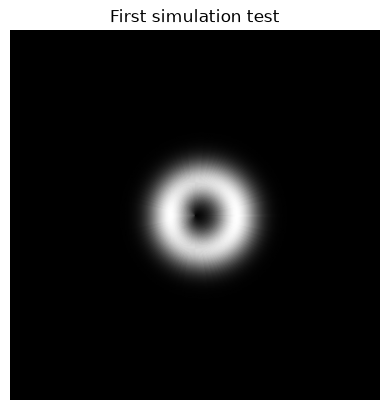

More Complete configuration¶

For the second test, we will keep the configuration in a TOML file. This tends to be easier to read than the dict in python code. The file is Demo01.toml, and we read it thus:

import tomllib as tl
with open( "Demo01.toml", 'rb') as f:
            toml = tl.load(f)
print( json.dumps( toml, indent=4 ) )

{
    "simulator": {
        "model": "Raytrace",
        "cropsize": 256
    },
    "lens": {
        "mode": "SIE",
        "einsteinradius": 46,
        "ellipseratio": 0.34,
        "orientation": 107
    },
    "source": {
        "mode": "SersicSphere",
        "sigma": 20,
        "sigma2": 10,
        "theta": 45,
        "position": "cartesian",
        "n_sersic": 4,
        "luminosity": 16
    },
    "position": {
        "x": 11.01,
        "y": 0.31
    }
}

The result is a nested python dict which we can import as we did before.

Most importantly, we are now defining simulator.model, lens.mode and source.mode which make the lens, source, and simulation models explicit. Specifically, we do raytrace simulation with a SIE lens lensing a spherical source with sersic light profile. The sersic parameters (n_sersic and luminosity) match the current defaults in the GUI.

In the run below, we set verbose=2 which gives extra diagnostic output. This is just to demonstrate the feature. It is only needed for debugging.

param = Parameters( toml )
imsim = SimImage( param, verbose=2 )
im = imsim.getImage()
plt.imshow( im, cmap='gray')
plt.title( "Simulation from TOML" )
plt.axis("off")

[GenericSim] init (verbose=2) ...
[SimulatorModel::getDistorted()]
[setDebug] 2

[SimImage] init (verbose=2) ...
[getSource] src=SersicSphere, ltprf0=None, verbose=2
[getSource] Lightprofile: SersicSphere LightProfileSpec.Sersic
[getSource] mode=SourceSpec.Sphere, ltprf=LightProfileSpec.Sersic
[getSource] Spherical Source - n_sersic=4.0, luminosity=16.0
[SphericalSource] constructor done
getSource() returns
[initSim] XY 11.01 0.31

[Source] Constructor
[SphericalSource] SERSIC
setFile /home/runner/.local/lib/python3.14/site-packages/CosmoSim/sie05.txt
[PsiFunctionLens.initAlphasBetas] Amplitudes file /home/runner/.local/lib/python3.14/site-packages/CosmoSim/sie05.txt
[initAlphasBetas] opened file /home/runner/.local/lib/python3.14/site-packages/CosmoSim/sie05.txt
[SimulatorMode::setLens] SIE
[SimulatorModel::setSource] setting source
[SimulatorModel::setNterms] 10 -> 5
[SimulatorModel::update] Lens: SIE
[Lens::getXi] [11.01, 0.31]
[Lens] Fix pt it'n 0; xi0=[11.01, 0.31]; Delta eta = 36.6416, -9.08535
[Lens] Fix pt it'n 1; xi0=[47.6516, -8.77535]; Delta eta = 35.7969, -20.7514
[Lens] Fix pt it'n 2; xi0=[46.8069, -20.4414]; Delta eta = 32.9541, -30.1972
[Lens] Fix pt it'n 3; xi0=[43.9641, -29.8872]; Delta eta = 29.7863, -35.9659
[Lens] Fix pt it'n 4; xi0=[40.7963, -35.6559]; Delta eta = 27.4199, -39.0343
[Lens] Fix pt it'n 5; xi0=[38.4299, -38.7243]; Delta eta = 25.9468, -40.6045
[Lens] Fix pt it'n 6; xi0=[36.9568, -40.2945]; Delta eta = 25.1042, -41.4085
[Lens] Fix pt it'n 7; xi0=[36.1142, -41.0985]; Delta eta = 24.6416, -41.8238
[Lens] Fix pt it'n 8; xi0=[35.6516, -41.5138]; Delta eta = 24.3926, -42.0401
[Lens] Fix pt it'n 9; xi0=[35.4026, -41.7301]; Delta eta = 24.26, -42.1533
[Lens] Fix pt it'n 10; xi0=[35.27, -41.8433]; Delta eta = 24.1898, -42.2127
[Lens] Fix pt it'n 11; xi0=[35.1998, -41.9027]; Delta eta = 24.1526, -42.2439
[Lens] Fix pt it'n 12; xi0=[35.1626, -41.9339]; Delta eta = 24.1331, -42.2603
[Lens] Fix pt it'n 13; xi0=[35.1431, -41.9503]; Delta eta = 24.1227, -42.269
[Lens] Good approximation: xi0=[35.1431, -41.9503]; xi1=[35.1327, -41.959]
[Lens::getXi] [11.01, 0.31] -> [35.1327, -41.959]
[setNu] etaOffset set to zero.
[SimulatorModel::update] Done updateApparentAbs()
[SimulatorModel::update] thread section
[Source::getImage()]
[SimulatorModel::updateInner()] eta=[11.01, 0.31]
[SimulatorModel::updateInner()] xi=[35.1327, -41.959]; eta=[11.01, 0.31]; etaOffset=[0, 0]
[SimulatorModel::updateInner()] nu=[35.1327, -41.959]
[calculateAlphaBeta] [[35.1327, -41.959]] ... 
[PsiFunctionLens.calculateAlphaBeta()] 5; 46 - [35.1327, -41.959]
[RaytraceModel] distort() SIE (Spherical Source)
[RaytraceModel] distort() SIE (Spherical Source)
[RaytraceModel] distort() SIE (Spherical Source)
[RaytraceModel] distort() SIE (Spherical Source)
Time to update(): 34 milliseconds
[Simulator] Centre Point (20.22,5.91) (Centre of Luminence in Planar Co-ordinates)
[getImage] centring from parameters: None
[crop] cropsize=256

(np.float64(-0.5), np.float64(255.5), np.float64(255.5), np.float64(-0.5))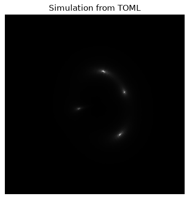

Comparing simulation models¶

For the simulation of SIE lenses, CosmoSim provides a total of four different simulation models

Raytrace is the exact simulation, as used above.
Roulette uses the Roulette formalism, which approximates using a local description of the lens potential

Each of these can also be run in a sampled version, where the lens potential is sampled and differentiated numerically, instead of using algebraic functions derived analytically.

To test different models, we can set simulator.model, which will override simulator.config, while keeping the SIE lens.

param["simulator"]["model"] = "Roulette"
param["simulator"]["nterms"] = 5
imsimRoulette = SimImage( param, verbose=0 )
imRoulette = imsimRoulette.getImage()
plt.imshow( imRoulette, cmap='gray')
plt.title( "Roulette Simulation" )
plt.axis("off")

[SimulatorModel::getDistorted()]
[Source] Destructor - destructed
[setDebug] 0

(np.float64(-0.5), np.float64(255.5), np.float64(255.5), np.float64(-0.5))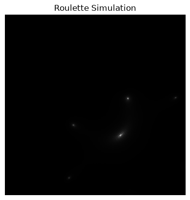

Because the source is small and provides little light, it is hard to distinguish the simulation models, but the critical point with Roulette is that it only provides a local description of the primary image. The secondary image on the far side of the lens will never appear in a roulette simulation.

We also see two spurious images, which are artifacts of the roulette formalism. There should be more, but they may be invisible because the source is faint. There should be a total of $n\pm1$ spurious images when $n$ roulette terms are used in the sum (nterms), forming a ring around the actual image and going through the centre of the lens.

Before we tamper with the source description, we will run sampled simulations as follows.

param["simulator"]["model"] = "Roulette"
param["simulator"]["sampled"] = True
imsimRouletteSampled = SimImage( param, verbose=0 )
imRouletteSampled = imsimRouletteSampled.getImage()

param["simulator"]["model"] = "Raytrace"
param["simulator"]["sampled"] = True
imsimRaytraceSampled = SimImage( param, verbose=0 )
imRaytraceSampled = imsimRaytraceSampled.getImage()

To better compare, we will show the four images side by side.

fig = plt.figure(figsize=(10, 10))
fig.tight_layout(pad=0.0)
plt.subplots_adjust(hspace=0.1, wspace=0.1) 

fig.add_subplot(2, 2, 1)
plt.imshow( imRouletteSampled, cmap='gray')
plt.title( "Sampled Roulette Simulation" )
plt.axis("off")

fig.add_subplot(2, 2, 2)
plt.imshow( imRaytraceSampled, cmap='gray')
plt.title( "Sampled Raytrace Simulation" )
plt.axis("off")

fig.add_subplot(2, 2, 3)
plt.imshow( imRoulette, cmap='gray')
plt.title( "Roulette Simulation" )
plt.axis("off")

fig.add_subplot(2, 2, 4)
plt.imshow( im, cmap='gray')
plt.title( "Raytrace Simulation" )
plt.axis("off")

(np.float64(-0.5), np.float64(255.5), np.float64(255.5), np.float64(-0.5))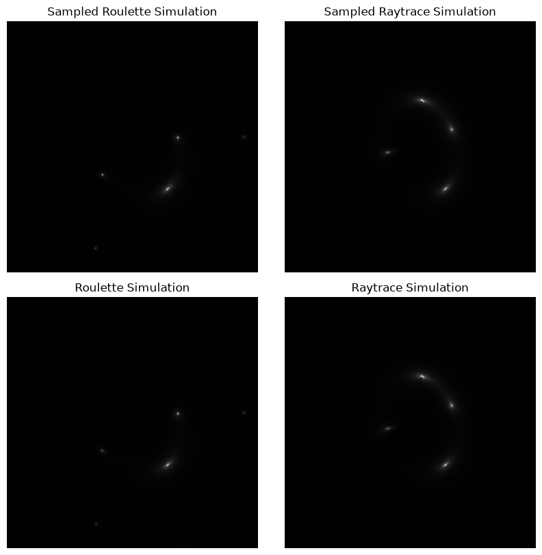

A convenience function¶

The following function does the four simulations and plots above, for any given set of parameters param. When we fiddle with the source (or lens) description, we will use this to run all tests at once.

def quadSim( param ):
    param["simulator"]["model"] = "Roulette"
    param["simulator"]["sampled"] = True
    imsimRouletteSampled = SimImage( param, verbose=0 )
    imRouletteSampled = imsimRouletteSampled.getImage()

    param["simulator"]["sampled"] = False
    imsimRoulette = SimImage( param, verbose=0 )
    imRoulette = imsimRoulette.getImage()

    param["simulator"]["model"] = "Raytrace"
    param["simulator"]["sampled"] = True
    imsimRaytrace = SimImage( param, verbose=0 )
    imRaytrace = imsimRaytrace.getImage()

    param["simulator"]["sampled"] = False
    imsimRaytraceSampled = SimImage( param, verbose=0 )
    imRaytraceSampled = imsimRaytraceSampled.getImage()

    fig = plt.figure(figsize=(10, 10))
    fig.tight_layout(pad=0.0)
    plt.subplots_adjust(hspace=0.1, wspace=0.1) 

    fig.add_subplot(2, 2, 1)
    plt.imshow( imRouletteSampled, cmap='gray')
    plt.title( "Sampled Roulette Simulation" )
    plt.axis("off")

    fig.add_subplot(2, 2, 2)
    plt.imshow( imRaytraceSampled, cmap='gray')
    plt.title( "Sampled Raytrace Simulation" )

    plt.axis("off")

    fig.add_subplot(2, 2, 3)
    plt.imshow( imRoulette, cmap='gray')
    plt.title( "Roulette Simulation" )
    plt.axis("off")
    
    fig.add_subplot(2, 2, 4)
    plt.imshow( imRaytrace, cmap='gray')
    plt.title( "Raytrace Simulation" )
    plt.axis("off")

    return( imRaytrace, imRoulette, imRaytraceSampled, imRouletteSampled )

The triangle source¶

The triangle source is specially designed for visual comparison of lensing configurations. This is what we get.

param["source"]["mode"] = "Triangle"
(im1,im2,im3,im4) = quadSim( param )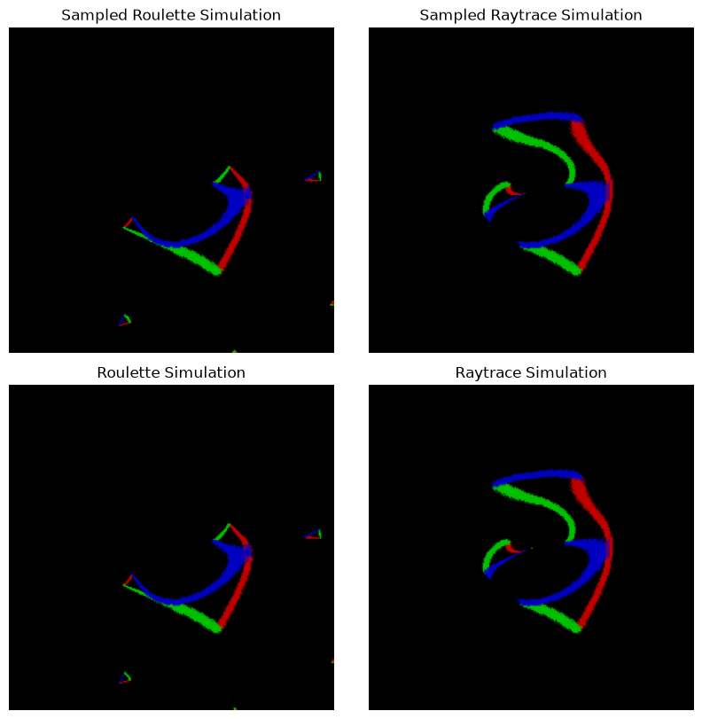

Since we stored the four images in variables (im1 through im4), we can also compare them using difference images. However, we have to take the range ( $0\ldots255$ ) into account when we calculate the difference. The following function does this

def imageDiff(im1,im2):
    im = (im1.astype(float) - im2.astype(float) + 256)/2 
    return im.astype(np.uint8)

Armed with the function, we can plot diff images.

fig = plt.figure(figsize=(14,7))
fig.tight_layout(pad=0.0)
plt.subplots_adjust(hspace=0.1, wspace=0.1) 

fig.add_subplot(1, 3, 1)
plt.imshow( imageDiff( im1, im3 ), cmap='gray')
plt.title( "Raytrace Simulation" )
plt.axis("off")

fig.add_subplot(1, 3, 2)
plt.imshow( imageDiff( im2, im3 ), cmap='gray')
plt.title( "Roulette Simulation" )
plt.axis("off")
    
fig.add_subplot(1, 3, 3)
plt.imshow( imageDiff( im4, im3 ), cmap='gray')
plt.title( "Sampled Roulette Simulation" )
plt.axis("off")

(np.float64(-0.5), np.float64(255.5), np.float64(255.5), np.float64(-0.5))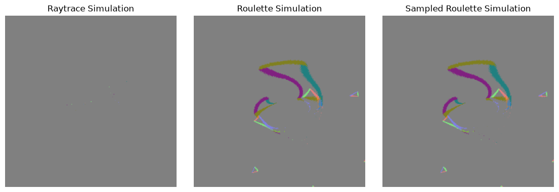

We see that the two raytrace simulations perfectly match, except for the tiny anomilty in the centre, which is probably due to the singularity of the lens potential at the origin.

The roulette simulations match well within the convergence ring.

What should concern us at the minute is the very small convergence ring for the unsampled roulette simulation. This does look wrong.

The number of Roulette terms¶

As mentioned, we cannot use more than five roulette terms with the SIE lens, but it is possible with sampled lenses. It is quite instructive to see how the image changes with the number of terms, so let’s try this.

param["simulator"]["nterms"] = 20
param["simulator"]["model"] = "Roulette"
param["simulator"]["sampled"] = True
im20 = SimImage( param, verbose=0 ).getImage()
csimg.imageCompare( im4, im20, "$n=5$", "$n=20$" )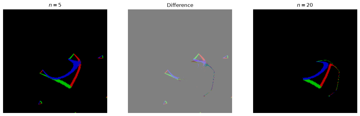

Here we compare five terms and twenty terms. We see that the few and large spurious images for $n=5$ are replaced by many small ones for $n=20$ . In this case, the spurious images only form a ragged half-ring, and not the smooth circle that we would have expected. This is probably due to numerical approximation.

Let’s compare with $n=10$ too, and add the axis cross so that we see the location of the lens.

param["simulator"]["nterms"] = 10
im10 = SimImage( param, verbose=0 ).getImage()
csimg.imageCompare( im4, im10, "$n=5$", "$n=10$", axiscross=True )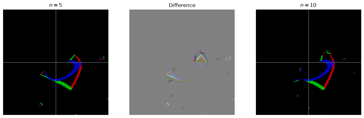

For $n=10$ we can clearly see the spurious images forming a ring.

Elliptic source¶

Finally, lets look at elliptic sources. We reset the simulator to Raytrace and SIE, and change the source to SersicEllipsoid.

param["simulator"]["model"] = "Raytrace"
param["source"]["mode"] = "SersicEllipsoid"
im1 = SimImage( param, verbose=0 ).getImage()
csimg.imshow( im1, "Elliptic Source" )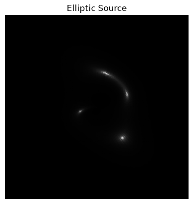

It may also be interesting to rotate the source differently

print( param.get( ("source","theta") ) )
param["source"]["theta"] = 90
im2 = SimImage( param, verbose=0 ).getImage()
csimg.imshow( im2 )

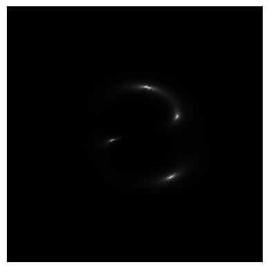
As we can see, different rotations make a massive difference to the observed image. However, this source is extremely longated.

Tip

To change the source size, we can use

param["source"]["sigma"] = 20
param["source"]["sigma2"] = 40

The parameter sigma refers to the standard deviation in a Gaussian light profile. Ellipsoid spheres have a size parameter along each axis, hence sigma and sigma2.

Closure¶

We have demonstrated the four basic simulation modes here, roulette and raytrace with and without sampling. This provides the cornerstone for further exploration.

We have also demonstrated some variation in sources, but we have still not discussed what makes reasonable parameters for lenses and sources.

The only lens we have considered is SIE. The other main alternative is SIS. Point Mass lenses are also implemented but not as thoroughly tested with newer features of CosmoSim. (As of 1 July 2026 with CosmoSim v3.1.0.)