Resimulation Template

This Demo assumes that you are familiar with the principles from Demo01.md. We start with the same imports

from copy import deepcopy

from CosmoSim.datagen import SimImage
from CosmoSim.roulettegen import Resim
import CosmoSim.Image as csimg
from CosmoSim import Parameters

import CosmoSim as cs
print( "CosmoSim version", cs.__version__ )

CosmoSim version 3.2.2b2

Basic Configuration¶

We start with parameters similar to the ones from Demo01.md, to make a baseline raytrace simulation using a SIE lens. We have just rounded some of the parameters to get neater numbers. We will use the simulation from SimImage to get roulette amplitudes for resimulation.

cfg = { "simulator" : {
            "model" : "Raytrace",
            "nterms" : 5,
            "centred" : False
      }
      , "lens" : {
            "mode" : "SIE",
            "einsteinR" : 50,
            "ellipseratio" : 0.4,
            "orientation" : 105
      }
      , "source" : {
            "mode" : "SersicEllipsoid",
            "sigma" : 10,
            "sigma2" : 30,
            "theta" : 45,
            "position" : "cartesian",
            "n_sersic" : 4,
            "luminosity" : 10
      }
      , "position" : { "x" : 12, "y" : 6 }
 }
param = Parameters( cfg )

Note that we have set centred=False. If we centre the image, we do not get a fair comparison between original roulette simulation and resimulation.

imsim = SimImage( param, verbose=0 )
im = imsim.getImage()
csimg.drawAxes( im )
csimg.imshow( im, "Baseline simulation" )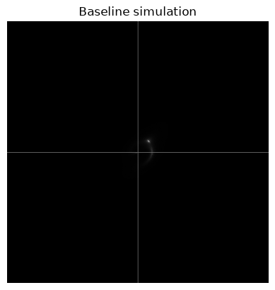

Roulette parameters¶

We can retrieve the roulette amplitudes with the getData() method. The resulting data is a pandas Series.

row = imsim.getData()
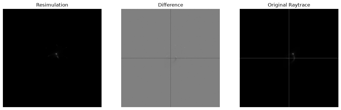
rsim = Resim( row, verbose=0 )
resimImage = rsim.getImage()
csimg.imageCompare( resimImage, im, "Resimulation", "Original Raytrace" )

[getSource] src=SersicEllipsoid, ltprf0=None, verbose=1
[getSource] mode=SourceSpec.Ellipse, ltprf=LightProfileSpec.Sersic

For reference, we can do the original roulette simulation, using a SimImage object.

roulettecfg = deepcopy( cfg )
roulettecfg["simulator"]["model"] = "Roulette"
roulettecfg["simulator"]["centred"] = False
rouletteparam = Parameters( roulettecfg )
roulette = SimImage( rouletteparam, verbose=0 )
rouletteImage = roulette.getImage()
csimg.imageCompare( resimImage, rouletteImage, "Resimulation", "Roulette simulation" )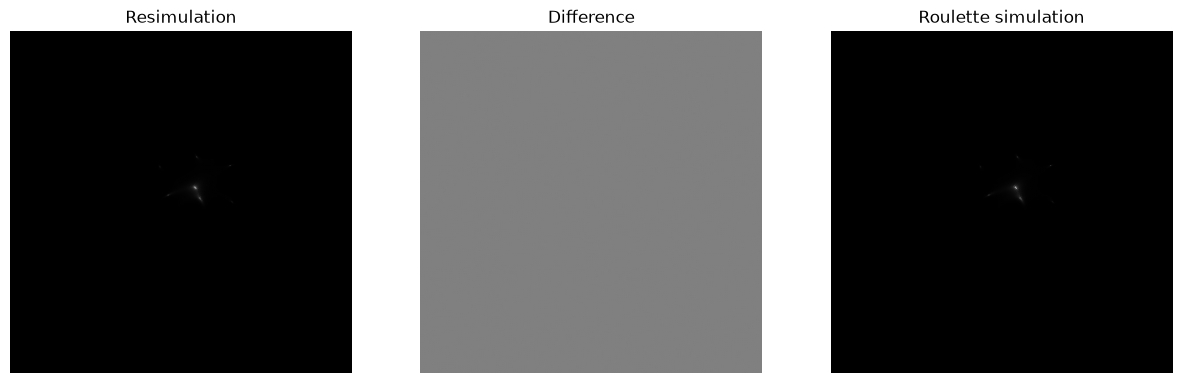

The two roulette simulations look similar but displaced compared to each other.

Further inspection¶

The Source¶

We can have a look at the original source image.

actual = rsim.getActualImage()
csimg.imshow( actual, "Actual source image" )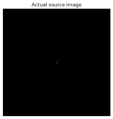

Data row¶

The data row retrived by getData() looks like this:

display( row )

filename              test.png
source         SersicEllipsoid
x                           12
y                            6
sigma                       10
sigma2                      30
theta                       45
lensX                        0
lensY                        0
centreX                      0
centreY                      0
reletaX                   12.0
reletaY                    6.0
offsetX               0.009262
offsetY              10.589655
xiX                  19.167676
xiY                   23.74807
alpha[0][1]                0.0
alpha[1][0]          -0.308419
alpha[1][2]          -0.065094
alpha[2][1]          -0.000926
alpha[2][3]           0.015552
alpha[3][0]          -0.000691
alpha[3][2]           0.001232
alpha[3][4]          -0.000755
alpha[4][1]           0.000037
alpha[4][3]          -0.000049
alpha[4][5]          -0.000053
alpha[5][0]          -0.000004
alpha[5][2]           0.000012
alpha[5][4]          -0.000013
alpha[5][6]           0.000018
beta[0][1]                 0.0
beta[1][0]                 0.0
beta[1][2]            0.301471
beta[2][1]            0.020228
beta[2][3]            -0.00282
beta[3][0]                 0.0
beta[3][2]           -0.000146
beta[3][4]           -0.000986
beta[4][1]            0.000116
beta[4][3]           -0.000112
beta[4][5]            0.000123
beta[5][0]                 0.0
beta[5][2]           -0.000014
beta[5][4]            0.000011
beta[5][6]           -0.000002
Name: test.png, dtype: object

Here we see that we have roulette amplitudes up to order 5, which is the maximum implemented for analytical SIE.