The roulette formalism describes the lens potential locally in a point, by a process similar to Taylor expansion. The description is given by a number of roulette amplitudes and , which can be calculated in (at least) two different ways:
Given the roulette amplitudes, it is also possible to simulate the distorted image in a neighbourhood of the reference point.
Simulation in the roulette formalism
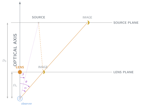
The figure shows the set-up for the flat-sky approximation, with the source plane (the lens plane) a distance () from the observer.
The observed lensing is decomposed into two steps, as shown by the figure. The first step is a translation (deflection), corresponding to the difference between apparent () and actual () source position:
We have already seen that the deflection angle may be expressed as the gradient of the two-dimensional projected lensing potential. In the roulette formalism this translates into a set of so-called roulette amplitudes. In particular
where is a vector of roulette amplitudes, as defined above.
The second step is the actual, non-linear distortion, and may be expresed through higher-order derivatives of the lensing potential. The distorted image is drawn in a local co-ordinate system in the lens plane, centred at . Following Clarkson, we use polar co-ordinates for the distorted image. While Clarkson used we will use , since we use angular units.
The source image is described in Cartesian co-ordinates centered at in the source plane.
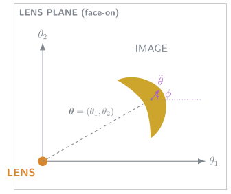
Figure 2:The lens plane, viewed face-on. The dashed vector gives the position of the image’s light centre (the small dot) relative to the lens. The local polar co-ordinate system is centred on this light centre, with the (angular) radius and the angle from the local polar axis (parallel to the global direction). The global coordinate directions , centred on the lens, are shown for reference.
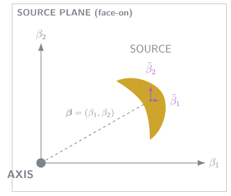
Figure 3:The source plane, viewed face-on. The dashed vector gives the position of the source’s light centre (the small dot) relative to the optical axis. The local Cartesian co-ordinate system is centred on this light centre, parallel to the global axes. The global coordinate directions , centred on the optical axis, are shown for reference.
Thus the light observed at a position (pixel) is drawn from a different position (pixel) in the source image. From Eq. (48) in Clarkson (2016) it is possible to show that the mapping is given as
The coefficients and depend on the lens potential , from which one may derive the physical properties of the lens.
In practice the sum has to be truncated by limiting for some .
The roulette amplitudes are always calculated in a specific Reference Point. In the next section we will give expressions for calculating the roulette amoplitudes.
- Clarkson, C. (2016). Roulettes: a weak lensing formalism for strong lensing: II. Derivation and analysis. Classical and Quantum Gravity, 33(24), 245003. 10.1088/0264-9381/33/24/245003